« 5.5: External Data |
6.2: Colour Channels »
In this tutorial, we’ll look at a few cool image processing techniques. You are already familiar with the image() function, which you’ve used in combination with loadImage() to draw image files to the display window. GIF, JPG, and PNG files are all raster graphics formats – that’s, digital images comprised of a pixel grid. We’ll look at reading values off individual- as well as groups of pixels and then manipulating them to create Photoshop-esque filters. To manage these arrays of pixel values, we’ll rely on a number of the techniques that you picked up in lesson 5, in particular, the combining of loops with lists.
To begin, we’ll peek under the hood of some image file formats; this will provide useful insight into how the colours of individual pixels are controlled.
Image Formats
Each time you run a sketch, Processing generates a new or updated display window. Like a GIF, JPG, or PNG image, the graphic presented in the display window is raster-based. Using the saveFrame() function one can capture the current frame in TIFF (.tif) format. Alternatively, a (filename) argument ending in .gif, .jpg, or .png produces a compressed image file. With TIFF, Processing employs no compression resulting in larger files. TARGA (.tga) is also an option, but these lessons avoid covering it in favour of focussing on the more common web-browser-supported formats.
Below is a screenshot of a sketch. The code is not important. Instead, focus on what the display window renders (a red and white striped pattern) and the file sizes of each version saved.
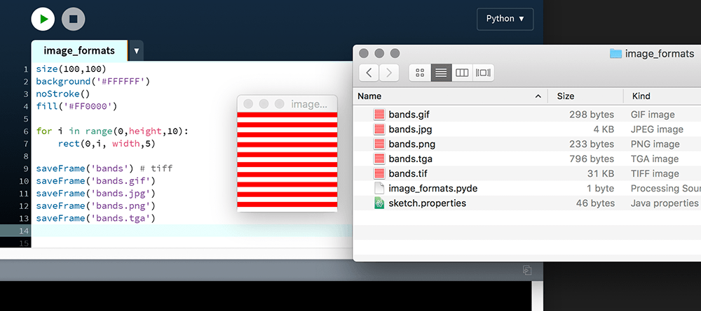
| bands.gif | – 298 bytes |
| bands.jpg | – 4 KB |
| bands.png | – 233 bytes |
| bands.tga | – 796 bytes |
| bands.tif | – 31 KB |
Before proceeding with an explanation for these differences, here’s a 3-point primer on file size:
- you know that computers store digital information as ones and zeroes; you refer to each 1 or 0 as a bit (a binary digit);
- there are 8 bits in a byte, for example,
10110110; - a kilobyte (KB) is 1000 bytes.
The “bands.tif” file is by far the largest, weighing in at a comparatively hefty 31 kilobytes. Recall that Processing uses no compression when saving TIFF files, so this is no surprise. But how exactly does a TIFF store pixel values, and what is the relation to size? To begin to answer this question, consider the hexadecimal value for red:
#FF0000
Each pair of digits has been coloured according to the RGB primary it controls. Alternatively, we could rewrite this using decimal values:
(255, 0, 0)
Alas, this still isn’t pure ones and zeroes. Information stored digitally requires conversion to binary. It figures, right? Because binary comprises ones and zeroes, and so do bits. To convert from a zero in decimal to a zero in binary is easy – it’s 0 in both systems. The same goes for 1. But what about 2? Binary has only two digits to work with, whereas decimal has ten. Below is an abridged conversion table:
| Decimal | Binary |
|---|---|
| 0 | 0 |
| 1 | 1 |
| 2 | 10 |
| 3 | 11 |
| 4 | 100 |
| 5 | 101 |
| … | |
| 255 | 11111111 |
We count on our fingers, so a base-10 (decimal) system is fitting. For instance, suppose you are counting the number of people who pass you in the street. To keep track, you begin by forming a fist with each hand; when the first person passes you, you raise your left thumb. For the second person, you extend your left index finger; and so forth. I know this seems menial but bear with me.

You reach ten people and have run out of fingers. For the eleventh passerby, you ask a friend sitting beside to ‘store’ a one on her fingers. You then close your fists beginning at one again (your left thumb). When you reach twenty, your friend extends her left index finger, and you start at one again. In all, twenty-six people pass you.

To proceed beyond a hundred with this system, you’ll need to find another friend. From this exercise, we gather that for each power of ten you require an additional digit – i.e. 10, 100, 1000.
Now, imagine you had no fingers (or thumbs). Once you’ve counted to two, you run out of ‘stumps’ to count on. When counting in binary (base-2), every time you reach some power of two an additional digit’s required. The table below provides binary-to-decimal conversions for powers of two.
| Binary | Decimal |
|---|---|
0 |
0 |
10 |
2 |
100 |
4 |
1000 |
8 |
10000 |
16 |
100000 |
32 |
... |
|
If you were using your friends to help hold digits, counting to 32 requires five assistants. Don’t worry, though, this conversion process is handled for you by Processing so that you’ll never need to deal directly with binary.
In lesson 1.2 you received little explanation for how hexadecimal actually works. You’ve probably been wondering where those letters from, right? Well, hexadecimal is a base-16 system. Just imagine some alien race with sixteen fingers. To accommodate these extra fingers, we include the letters A to F.
| Hexadecimal | Decimal |
|---|---|
... |
|
8 |
8 |
9 |
9 |
A |
10 |
B |
11 |
C |
12 |
D |
13 |
E |
14 |
F |
15 |
10 |
16 |
11 |
17 |
... |
|
FF |
255 |
People have used all sorts of numeral systems. For example, the French use base-10 until seventy, after which point it’s a mixture of base-10 and base-20. The Telefol and Oksapmin speaking people of Papua New Guinea use a Heptavigesimal (base-27) system, where the words for each number are named according to the 27 body parts they use for counting.
If you are wondering, π is irrational in every numeral system. But, on second thought, what if 3.141… were the base? 😕
Let’s return to binary numbers. Here are a few sequences:
| Binary | Decimal |
|---|---|
10000000 |
128 |
10000001 |
129 |
10000010 |
130 |
... |
|
11111111 |
255 |
100000000 |
256 |
Note how 255 is the highest decimal that can be represented using eight bits. It’s no coincidence that you express the brightest red your screen can display as (255, 0, 0). Or that white is (255, 255, 255). At a hardware level, these integers are all converted to binary. As indicated in the table above, eight 1s in binary is equivalent to 255 in decimal. Let us rewrite red in binary:
111111110000000000000000
I have padded the green and blue values with zeroes so that each colour is eight bits in length. White would be a complete string of ones. In all, there are 8 × 3 = 24 bits. Hence, this is 24-bit colour, which can describe a whopping 256 × 256 × 256 = 16,777,216 possible (yet not necessarily distinguishable) colour variations.
Now, back to the sketch. To remind you, this the visual output we are dealing with:

The size of the (uncompressed) TIFF file is 31 KB. Here’s why:
- the graphic is 100 pixels wide by 100 pixels high, and therefore comprised of 100 × 100 = 10,000 pixels;
- each pixel contains one 24-bit colour value;
- 10,000 pixels × 24-bit colour values = 240,000 bits;
- there are 8 bits in a byte, so that’s 240,000 bits ÷ 8 = 30,000 bytes.
- 30,000 bytes = 30 kilobytes (KB).
Okay, so we have accounted for 30 KB, but what about the extra 1 KB? I have used Hex Fiend – an open source hex editor – to open and inspect the raw data of the “bands.tif” file. Of course, the data is ultimately stored as binary, but it’s easier to make sense of hexadecimal. You can follow along using a hex editor too, but there’s no need.
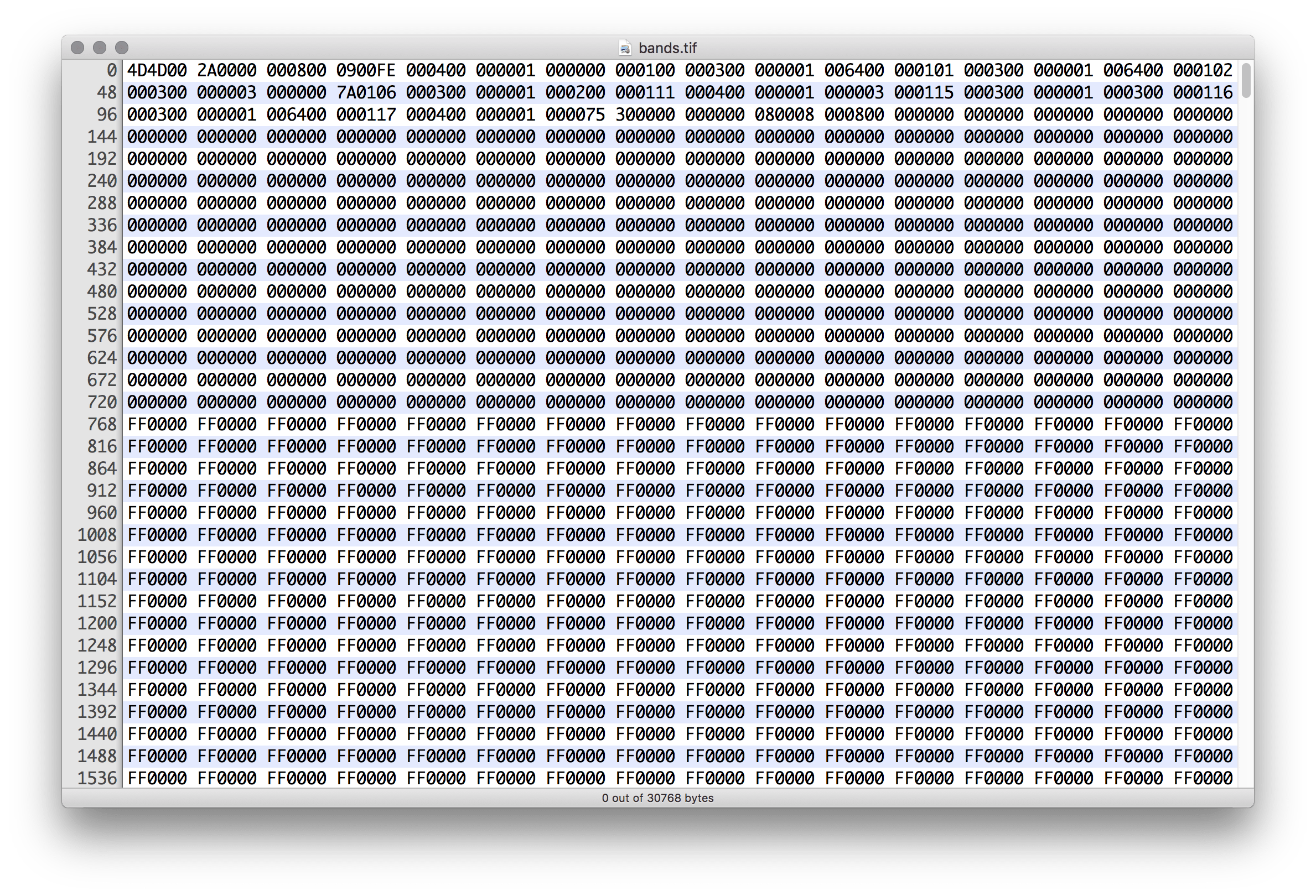
FF0000 and FFFFFF values.The numbers appear in byte groupings of three (clusters of six 0–F numbers). Scrolling through the file reveals alternating stretches of FF0000 and FFFFFF values – that’s, red and white respectively; this is what we would expect, after all, the graphic is a pattern of alternating white and red stripes. However, the first three lines contain a bunch of seemingly random numbers; then, there are 000000s (black?) up to byte 768 (as indicated by the count in the left margin).
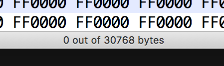
FF0000 or FFFFFF values. The first stretch of FF0000's appear at byte 768.At the bottom of the window, you can spot the file size in bytes.
that’s 768 bytes over our expected 30,000. This accounts for the extra 1 KB, which the file manager has rounded-up to 31 KB. Removing everything up to where the first FF0000 cluster reduces the file size to precisely 30 KB.
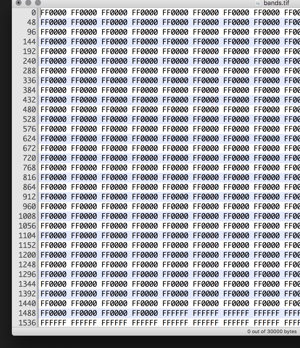
FF0000 instance leaves you with a file of 30,0000 bytes.So what was stored in bytes 0 to 768? The beginning section of the file contains vital information to identify it as a TIFF and specify parameters for – but not limited to – width, height, bit-depth, and orientation. Leaving this information out will most certainly break the graphic.
Processing generates TIFF files using the format’s most essential features. The TIFF 6.0 specification can support various compression schemes, layers, deep colour (16- as opposed to 8-bits per channel), transparency, pages, and multiple colour models (RGB, CMYK, LAB, etc.). Be aware, though, that many of these extra features are extensions, and reader support will vary. Overall, TIFF is a very versatile format, well suited for working on graphics between different applications and for archiving purposes. Essentially, TIFF rolls all of GIF, JPG, and PNG’s features into a single specification. Nevertheless, it’s not supported on the Web.
GIF vs JPG vs PNG
If you are looking at an image on a web-page, chances are it’s either a GIF, JPG, or PNG. Scalable Vector Graphic format (SVG) is also popular, but not designed for raster graphics. Size is important to consider when you are transferring files across an internet connection. Smaller equals faster, so all three formats employ compression techniques.
The details of data compression are complicated, mathematical, and beyond the scope of these lessons. Nonetheless, you’ll gain a high-level insight into how compression algorithms operate. The main focus, though, is on why you’d elect to use one format over the other. If you are familiar with some raster editing software, such as GIMP or Photoshop, it’s a good idea to play around with the export options to see how the different GIF, JPG, and PNG parameters affect the quality and size of these files.
GIF
GIF is the oldest of the three formats. There’s an ongoing war over whether it’s pronounced “gif” (with a hard g, like in gift) or as “jiff”. The format utilises the Lempel–Ziv–Welch (LZW) data compression scheme. Our image is a sequence of red and white stripes, and this is just the type of graphic to which GIF is best suited. More specifically, images consisting primarily of areas filled in flat colour. For instance, graphs, diagrams, text, and line art. Unsurprisingly, it outperforms JPG and PNG for our red-white stripy pattern, consuming just 298 bytes. Opening the “bands.gif” file in a hex editor reveals how small it’s, and also provides insight into how the format works.
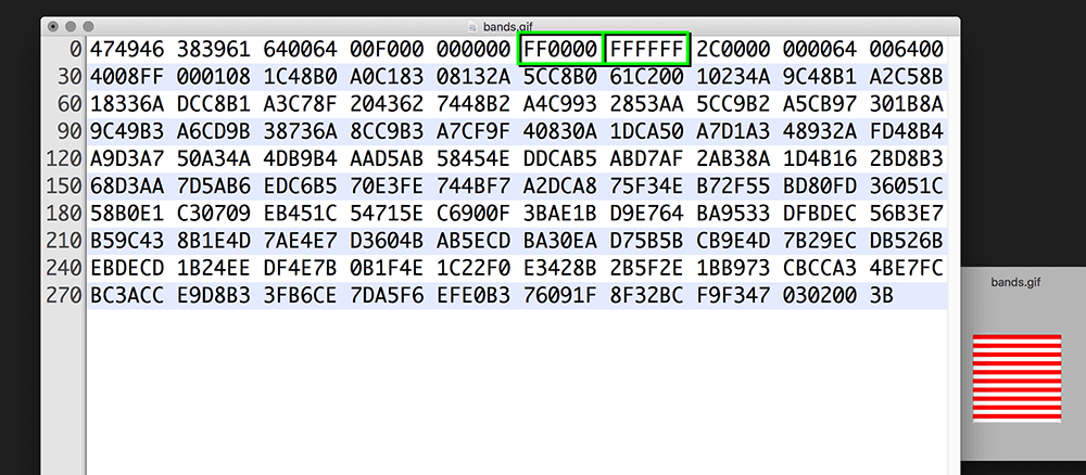
FF0000) and white (FFFFFF) have been outlined in green.Despite there being thousands of red and white pixels in the graphic, the hex editor contains a single instance of FF0000 and FFFFFF. This pair of colour values makes up the image’s colour table. What precedes the colour table identifies the file as GIF and describes the width, height, and other characteristics. What follows the colour table (after the 2C and terminating with a 3B) is compressed graphics data. Rather than specifying the value of each pixel, the LZW algorithm matches each pixel with one of the two colour table entries. But LZW can take this indexing system one step further. Each red stripe is a continuous string of 100 × 10 = 1000 hexadecimal values. This string can in-turn be stored in a table, so that each time the red stripe reappears, the relevant table entry is repeated.
GIF has its limitations. Most notably, the colour table may not exceed 256 colours. For greater GIF compression one reduces this palette further. The GIF below consists of around sixteen colours and the reduction in range is quite evident. Placing alternating colours in checkerboard-type arrangements – called dithering – helps make up for the limited colour table, but it’s often easy to discern this pattern, and it works against the compressibility. GIF supports transparency, but the level of opacity is either 0% or 100% (nothing between).
GIF also supports animation, which is handy for short loops of cats doing silly things.
JPG
JPG (pronounced “jay-peg”; often bearing the extension .jpeg) uses a lossy compression that does not support any type of transparency. Unlike lossless GIFs or PNGs, each time you reopen, perform a minuscule edit, and save a JPG file, the image quality degrades further. The compression algorithm works by taking advantage of the human psychovisual system, disregarding information we are less likely to detect visually. Humans are more sensitive to differences in brightness than differences in colour, a characteristic that JPG leverages. The format works well for images with graduated colour, like photographs, but causes noticeable artefacts to appear wherever there’s a sharp contrast.
Most raster software provides some or other of quality ‘slider’ when exporting to JPG format. Less quality equals smaller file size, but you’ll find that certain photographs/graphics can handle more compression before they begin to look horrible.
PNG
PNG – pronounced “pee-en-jee” or “ping” – was developed as a replacement for the proprietary GIF format. Although GIF patents expired in 2004, PNG had introduced a number of compelling improvements. Like GIF, PNG compression is lossless, but the PNG with no 256 colours palette restriction. Moreover, transparency can range from anywhere between 0% to 100%, allowing for semi-opaque pixels. This is accomplished using an additional alpha channel. For instance, an opaque blue (i.e. no alpha) can be expressed as:
0000FF
Or, in binary:
000000000000000011111111
that’s 24 bits in all – with 8 bits for each R/G/B channel. A 32-bit hexadecimal value provides room for the additional alpha channel; of course, this consumes more storage/bandwidth too. The same blue with an opacity of around 25% is, hence, stored as:
00000000000000001111111101000001
This alpha feature is especially handy for placing images seamlessly above other background images.
Notably, PNGs do not support animation. The APNG (Animated Portable Network Graphics) specification is an extension to the format, but it has failed to gain traction with some major (Microsoft) web browsers.
When dealing with photographs, JPGs tend to trump PNGs in terms of quality-for-size. PNGs, however, excel when you require transparency or desire GIF-style sharpness with a greater range of colour.
There are a few up-and-coming Web image formats (WEBP, HEIC) that promise comparable quality in smaller files. Whether they gain traction depends largely on support from authoring tools and browsers. To reiterate, though, it’s best to experiment with the different formats to see how they work and which is most appropriate for a given graphic you wish to optimise.
6.2: Colour Channels »
Complete list of Processing.py lessons