« 3.4: Randomness |
4.2: Transformations »
In this tutorial, you get to make things move. The content focuses primarily on animation, but also covers transformations, time & date functions, and some trigonometry. As you’ll discover, blending motion with math produces some exciting results.
Animation
Before writing any animation code, consider how motion is perceived. The brain is fed a snapshot from your retina around ten times each second. The speed at which objects appear to be moving (or not moving) is determined by the difference between successive snapshots. So, provided your screen can display a sequence of static images at a rate exceeding ten cycles per second, the viewer will experience the illusion of smooth flowing movement. This illusion is referred to as Beta movement and occurs at frame rates of around 10-12 images per second – although higher frame rates will appear even smoother. That said, there’s more to motion perception than frames per second (fps).
Take a moment to note the numbering sequence of the circles in the illustration below.

Consider that you displayed just circle 1 for a full four seconds, followed by just circle 5 for another four seconds, looping the sequence indefinitely (an effective frame rate of 0.25 fps). The result, most observers would agree, is a pair of alternating images depicting circles in different positions. However, speed up the frame rate to around 2.5 fps, and one begins to interpret the sequence as a circle bouncing between two points. Speed up the frame rate further, and the two circles seemingly flicker in sync.
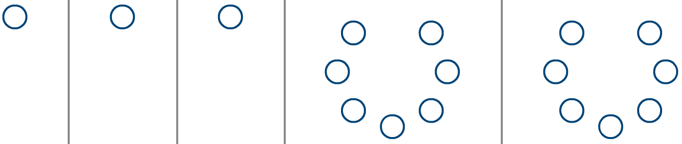
Frame rates from left to right: 0.25 fps; 2.5 fps; 12 fps; 1 fps; 25 fps
The two rightmost animations (rings of circles) run at 1 and 25 fps. In the left/slower instance, the circle just ahead of a gap appears to jump into the void left by the vacant circle (if you didn’t see it this way before, you should now). In the more rapid animation, a phantom white dot appears to obscure the circles beneath it as it races around the ring – an illusion referred to as the phi phenomenon.
Animation Functions
All that’s required to get animating in Processing are the setup() and draw() functions. Create a new sketch; save it as “beta_movement”; then add the following code:
def setup():
    size(500,500)
    background('#004477')
    noFill()
    stroke('#FFFFFF')
    strokeWeight(3)
The code resembles just about every other sketch you’ve set up thus far, excepting the def setup() line. Everything indented beneath the setup() is called once when the program starts. This area is used to define any initial properties, such as the display window size. Conversely, code indented beneath a draw() function is invoked with each new frame. Add a draw() function to see how this operates:
def setup():
size(500,500)
background('#004477')
noFill()
stroke('#FFFFFF')
strokeWeight(3)
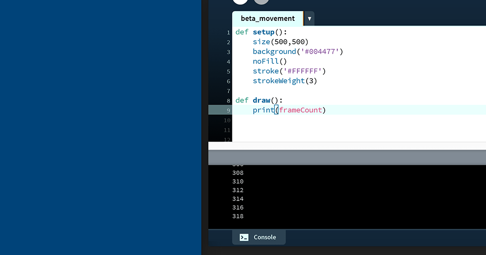
def draw():
print(frameCount)The frameCount is a system variable containing the number of frames displayed since starting the sketch. With each new frame, the draw() function calls the print function, which in-turn displays the current frame-count in the Console:
By default, the draw() executes at around 60 fps – but as the complexity of an animation increases, the frame rate is likely to drop. Adjust the frame rate using the frameRate() function (within the indented setup code), and add a condition to print on even frames only:
def setup():
    frameRate(2.5)
    size(500,500)
    background('#004477')
    noFill()
    stroke('#FFFFFF')
    strokeWeight(3)

def draw():
    if frameCount%2 == 0:
        print(frameCount)
With the frameRate set to 2.5, the draw line runs two-and-a-half times every second; this means each frame is 400 milliseconds (0.4 of a second) in duration. Because the print line executes on every second frame, a new line appears in the Console every 800 milliseconds:

To draw a circle on every even frame, add an ellipse() line:
def draw():
    if frameCount%2 == 0:
        #print(frameCount)
        ellipse(250,140, 47,47)
Now run the code. You may be surprised to find that the circle does not blink:

So why does the circle not disappear on odd frames? The reason is that everything in Processing persists after being drawn – so, every second frame another circle is drawn atop the existing ‘pile’. The background colour is defined within the setup() section, and is therefore drawn once; as it’s drawn first, it’s also the bottommost layer of this persistent arrangement. To ‘wipe’ each frame before drawing the next, simply move the background('#004477') line to your draw() section:
def setup():
    frameRate(2.5)
    size(500,500)
    noFill()
    stroke('#FFFFFF')
    strokeWeight(3)

def draw():
    background('#004477')
    if frameCount%2 == 0:
        #print(frameCount)
        ellipse(250,140, 47,47)
The result is a blinking circle. Using an else statement, add another circle with which this alternates:
def draw():
    background('#004477')
    if frameCount%2 == 0:
        #print(frameCount)
        ellipse(250,140, 47,47)
    else:
        ellipse(250,height-140, 47,47)
You can now adjust the frame rate to test the effects.
For a more convincing effect, the animation should fill-in the intermediate frames.

To accomplish this without having to write out each frame position, one requires a variable to store and update the circle’s y value.
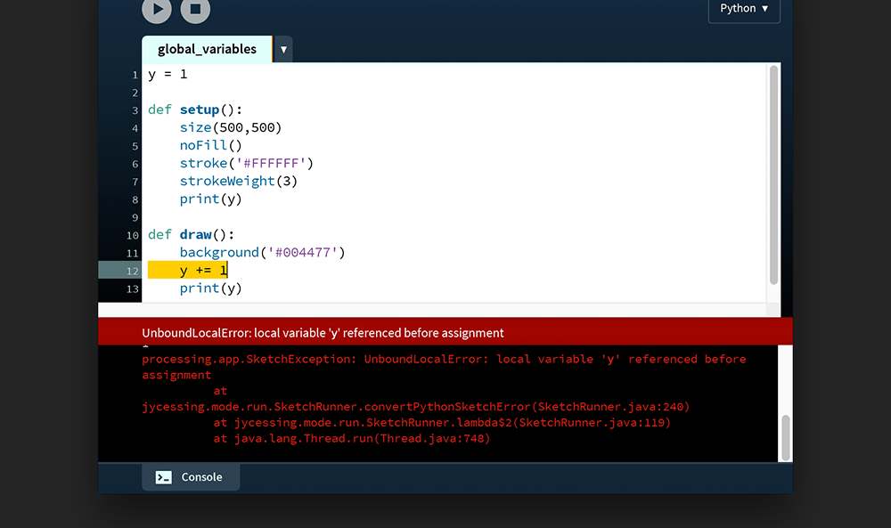
Global Variables
You’ll notice that the setup() and draw() functions are preceded by the def keyword. You’ll come to understand why this is in future lessons, but for now, need to be aware that variables cannot be directly shared between these two sections of code. Global variables address this challenge.
Create a new sketch and save it as “global_variables”. Add the following code:
def setup():
    size(500,500)
    noFill()
    stroke('#FFFFFF')
    strokeWeight(3)
    y = 1

def draw():
    background('#004477')
    print(y)
Run the sketch and note the error message:
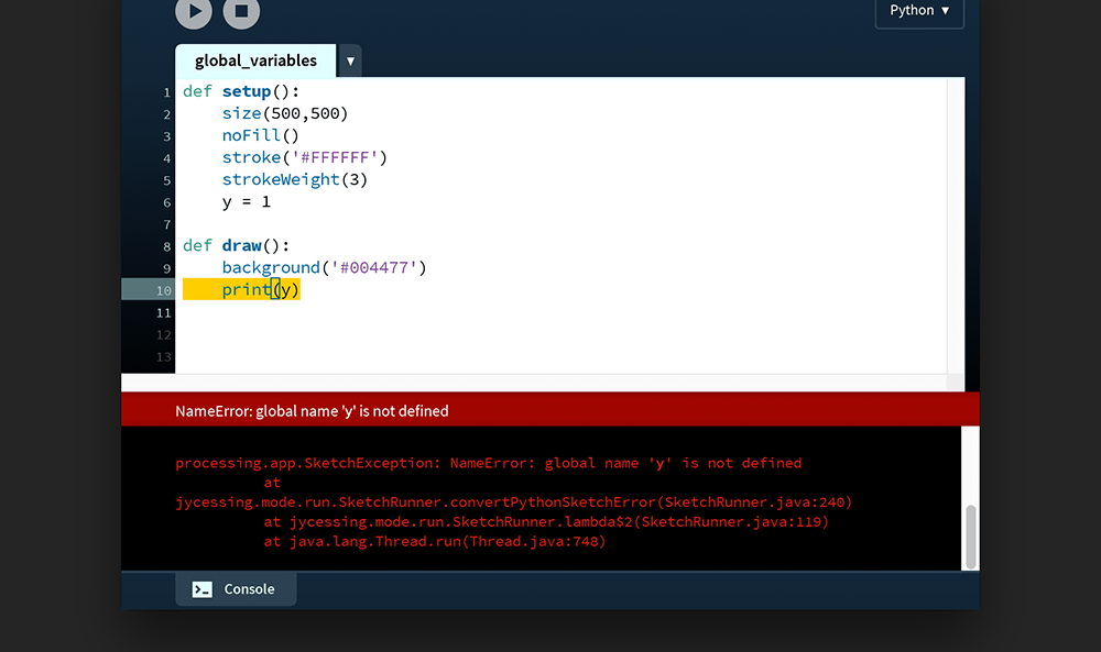
The y variable is defined within the setup() function. As such, y is only accessible among the indented lines of this block. The variable scope is therefore said to be local to setup(). Alternatively, one can place this variable line outside of the setup() function – thereby setting it in the global scope. This permits either function to read it. Stop writing code for a moment and consider the scenarios that follow.
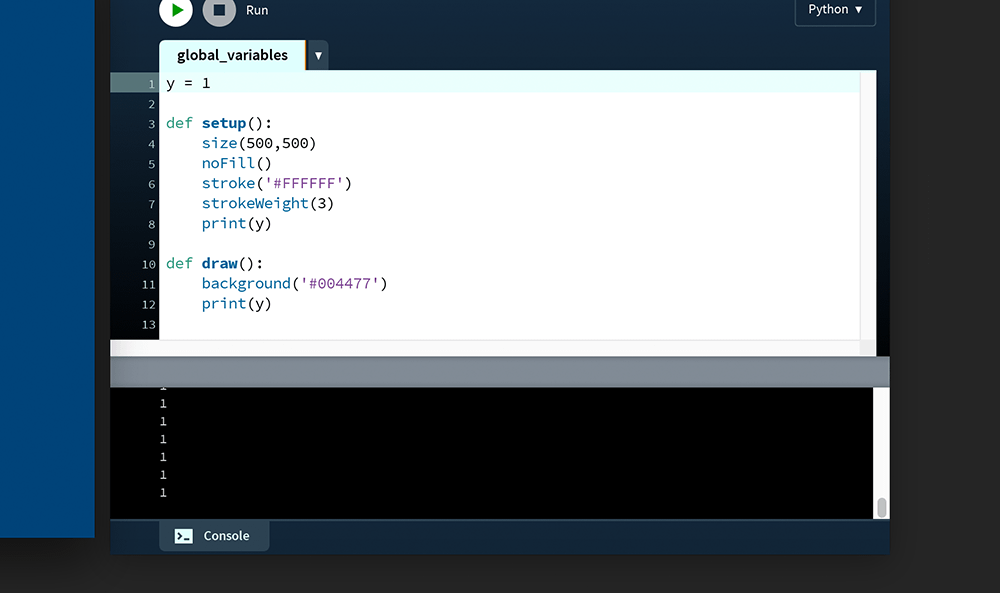
Adding the y = 1 line to the top of the code places the variable in the global scope, making it accessible to the setup() and draw() functions:
However, this global y variable can be overridden on a local level by another variable named y. In the example below, the setup() function displays a 1, whereas the draw() function displays zeroes:

1.While you can override a global variable, you’ll find that you cannot write/reassign a value to it:
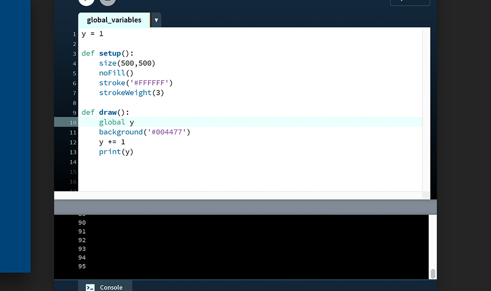
This is the point where the global keyword is useful. Edit your code, moving the y = 1 line to the top of your code (into the global scope). Then, to modify this variable from within the draw() function, bind it to the draw’s local scope using the global keyword:
y = 1

def setup():
    size(500,500)
    noFill()
    stroke('#FFFFFF')
    strokeWeight(3)
    print(y)

def draw():
    global y
    background('#004477')
    y += 1
    print(y)
The global y variable is now incremented by 1 with each new that’s frame drawn.
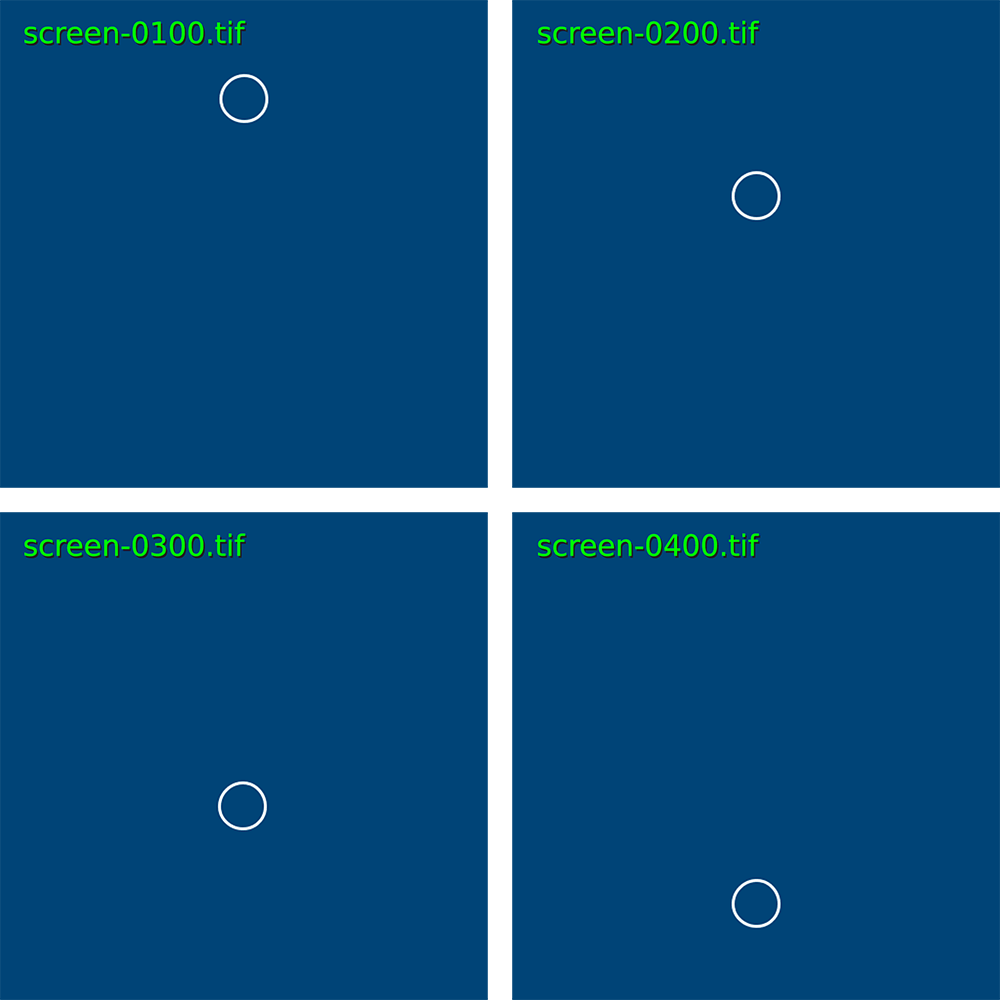
Add an ellipse() function to create an animated circle, the y-coordinate of which is controlled by the y variable:
def draw():
    global y
    background('#004477')
    y += 1
    print(y)
    ellipse(height/2,y, 47,47)
Run the code. In the graphic below, a motion trail has been added to convey the direction of motion.

Saving Frames
Processing provides two functions to save frames as image files: save() and saveFrame(). The latter is more versatile, so I won’t cover save().
Each time the saveFrame() function is called it saves a TIFF (.tif) file within the sketch folder, naming it using the current frame count. Add the following code to save every hundredth frame:
    ...
    ellipse(height/2,y, 47,47)

    if frameCount % 100 == 0:
        saveFrame()
Run the code and monitor the sketch folder. As every hundredth frame is encountered, a new file appears named “screen-” followed by a four-digit frame count padded with a leading zero(s).
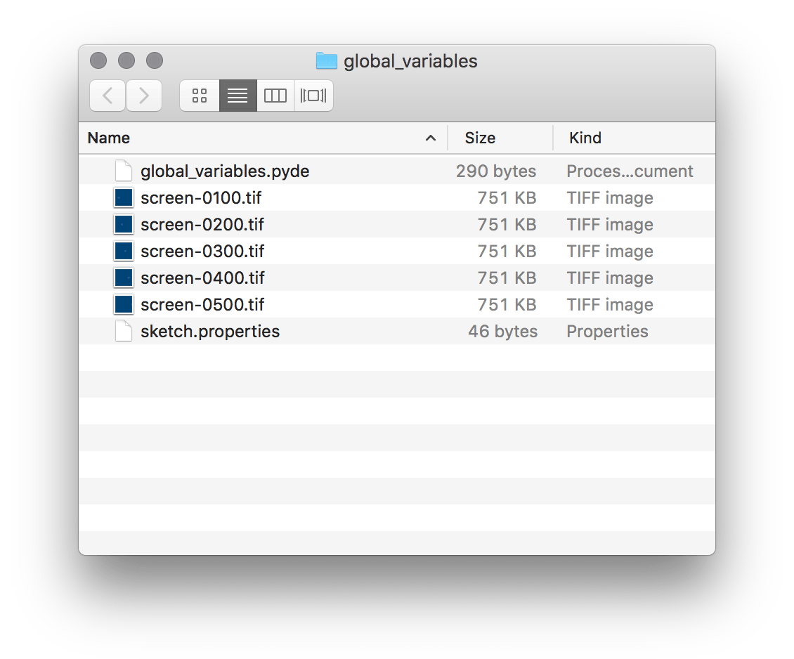
If you wish to save the file using a different name, and/or in some format other than TIFF – such as JPEG, PNG, or TARGA – refer to the saveFrame() reference entry.
DVD Screensaver Task
DVD players commonly feature a bouncing DVD logo as a screensaver, appearing after a given period of inactivity. You may also have seen some variation of this on another digital device, albeit with a different graphic. Intriguingly, people often find themselves staring at the pointless animation in the hope of witnessing the logo land perfectly in the corner of the screen. If you’re interested to know how long you can expect to wait for such an occurrence, refer to this excellent Lost Math Lessons article.
Create a new sketch and save it as “dvd_screensaver”. Within this, create a “data” folder. Download this “dvd-logo.png” file and place it in the data folder:
Add the following code:
x = 0
xspeed = 2
logo = None

def setup():
    global logo
    size(800,600)
    logo = loadImage('dvd-logo.png')

def draw():
    global x, xspeed, logo
    background('#000000')
    x += xspeed
    image(logo, x,100)
The only the unfamiliar line is the logo = None. This line defines the logo variable as an empty container in the global scope, which is then assigned a graphic in setup() function. Run the sketch.
DVD Forum [Public domain / filled in blue], from Wikimedia Commons
The logo should begin moving at an angle, rebounding off every wall it encounters. Your challenge is to complete the task.
Perhaps consider randomising the starting angle.
4.2: Transformations »
Complete list of Processing.py lessons