Processing.py in Ten Lessons – 4.2: Transformations

Transformations

Processing’s transform functions provide a convenient means of dealing with complex geometric transformations. Such operations include scaling, rotation, shearing, and translation. Suppose that you wish to rotate and scale the star shape depicted at the top-left, such that it results in the bottom-right:

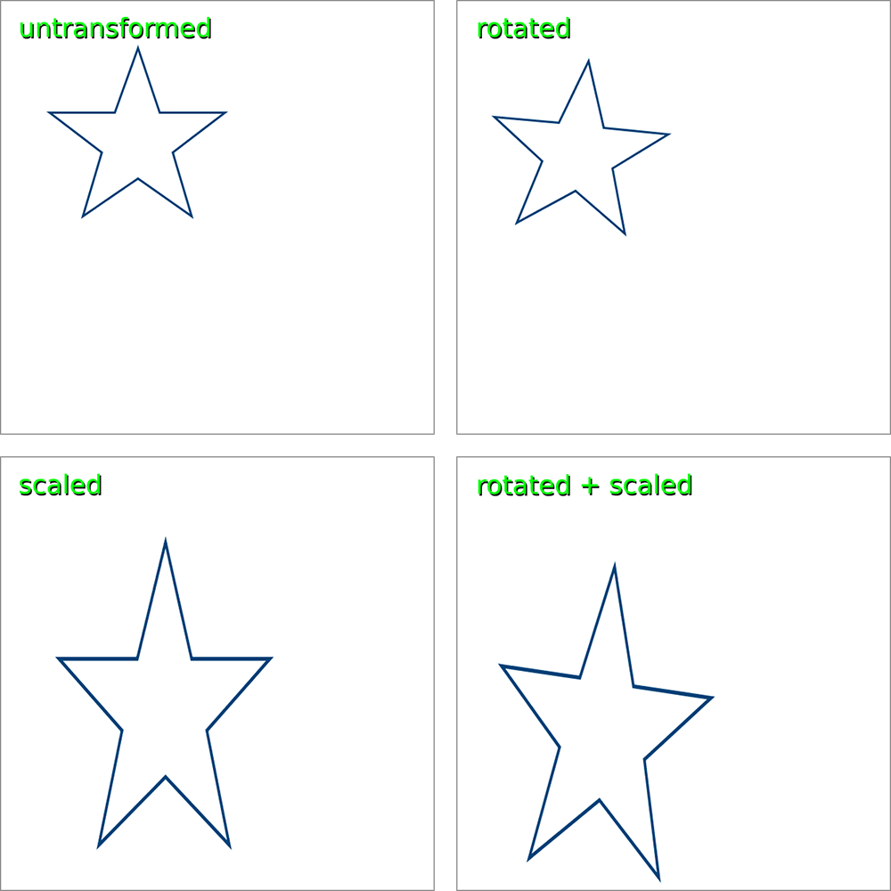
The code for the untransformed star’s ten vertices look something like this:

beginShape()
vertex(190,66)
vertex(220,155)
vertex(310,155)
vertex(238,210)
vertex(264,298)
vertex(190,246)
vertex(114,298)
vertex(140,210)
vertex(68,155)
vertex(158,155)
endShape(CLOSE)

To calculate the coordinates for the rotated + scaled vertex positions, a matrix is required.

Matrices

In mathematics, a matrix (plural: matrices) is a rectangular array of values. As an example, here’s a two-by-three matrix (2 rows, 3 columns):

[\begin{matrix} 2 & 5 & 12 \\ 19 & 9 & 7 \end{matrix}]

Given that digital images are essentially rectangular grids of pixels, it’s easy to imagine how matrices are used extensively in graphics processing. That said, matrices are applied in various fields of mathematics and other sciences.

To step you through how matrices operate, we’ll take a look at a few practical examples. Things get pretty mathematical here, but the idea is to grasp a matrix as a concept. Following this section, you’ll be introduced to Processing’s built-in matrix functions – meaning you’ll no longer need to perform the calculations yourself.

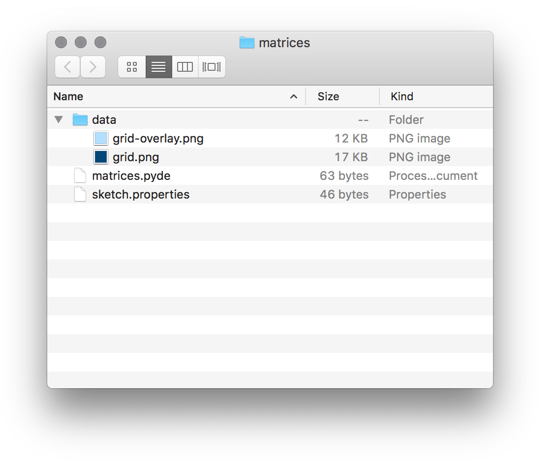
Create a new sketch and save it as “matrices”. Within the sketch’s folder, create a “data” subfolder containing a copy of the grid.png and grid-overlay.png files:

grid.png
grid-overlay.png

Add the following code:

size(800, 800)
grid = loadImage('grid.png')
image(grid, 0,0)
noFill()
stroke('#FFFFFF')
strokeWeight(3)

x = 400; y = 200
w = 200; h = 200

rect(x,y, w,h)

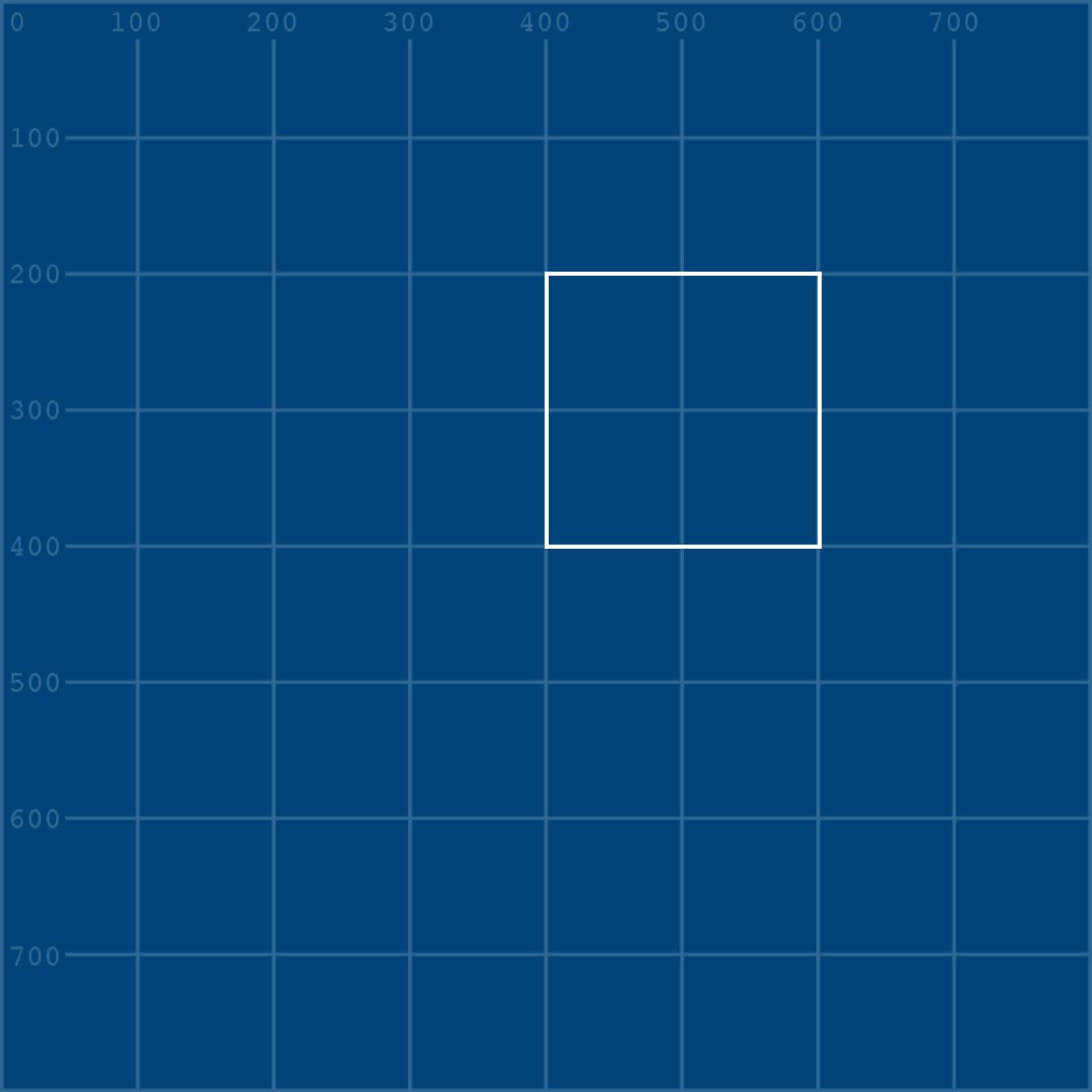
In Python, semicolons (;) serve as a substitute for new lines. The x/y/w/h variable assignments have been arranged in the above manner as a matter of style. If you wish to avoid the semicolons, you may write each variable on its own line. The x/y values represent the coordinates for the top-left corner of the square; the w/h variables, its width and height. Run the sketch and confirm that your display window matches the image below.

Matrices operate on vertices, whereas the rect() function does not. To move forward, substitute the rect() function with a quad().

#rect(x,y, w,h)
quad(
  x, y,
  x, y+h,
  x+w, y+h,
  x+w, y
)

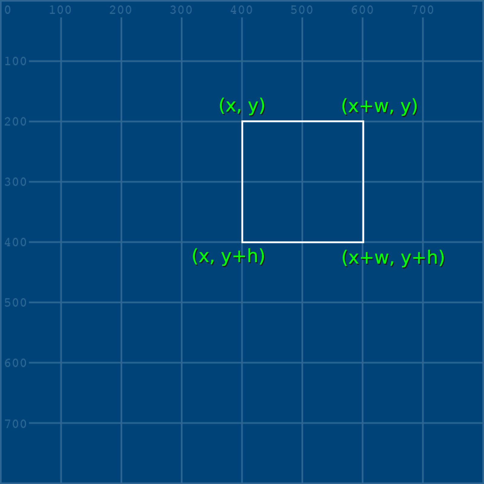
Vertices labelled according to their `quad()` arguments.

The output appears the same but is now based on vertices. Of course, this code does not make use of Processing’s vertex() function, but each x-y pair of values comprises a vertex nonetheless.

Translate

The first transformation you’ll perform is a translation; this involves moving the square a given distance in some direction. It’s an easy enough task to accomplish without a matrix, but also ideal for introducing how matrices work.

Firstly, take note of how the top-left vertex (x, y) determines the positions of the other three vertices. Therefore the only matrix operation you need to perform is on the top-left vertex – the remaining vertices can be calculated by adding the relevant w and h values. The matrix you are manipulating can, hence, be expressed as:

[\begin{matrix} x \\ y \end{matrix}]

Or, if you substitute the variable values:

[\begin{matrix} 400 \\ 200 \end{matrix}]

To translate a matrix, add (or subtract) another matrix. To perform a matrix addition, add-up the values of each row:

[\begin{matrix} x \\ y \end{matrix}] + [\begin{matrix} a \\ b \end{matrix}] = [\begin{matrix} x + a \\ y + b \end{matrix}]

Append the following code – namely: two new variables representing values a and b (the distance the shape must move horizontally and vertically); a yellow stroke; and a new quad() that integrates the matrix calculations within its arguments:

a = 100; b = -80
stroke('#FFFF00')
quad(
  x+a, y+b,
  x+a, y+h+b,
  x+w+a, y+h+b,
  x+w+a, y+b
)

Expressed in matrix notation, this is:

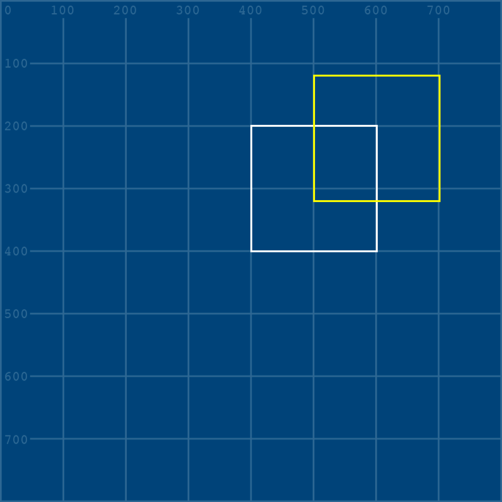
[\begin{matrix} 400 \\ 200 \end{matrix}] + [\begin{matrix} 100 \\ -80 \end{matrix}] = [\begin{matrix} 400 + 100 \\ 200 + -80 \end{matrix}]

Run the sketch. The new yellow square is drawn 100 pixels further right and 80 pixels closer to the top edge than the original.

Scale

To scale a shape, one must multiply the matrix you intend to transform by one describing a transformation. In mathematical notation, this can be expressed as:

[\begin{matrix} x \\ y \end{matrix}] \times [\begin{matrix} a & b \\ c & d \end{matrix}]

And this is the point where the power of matrices becomes evident! Depending on the values you substitute for a, b, c, and d, the result will be either a scale, reflect, squeeze, rotate, or shear operation. Take a moment to study how matrix multiplication is performed:

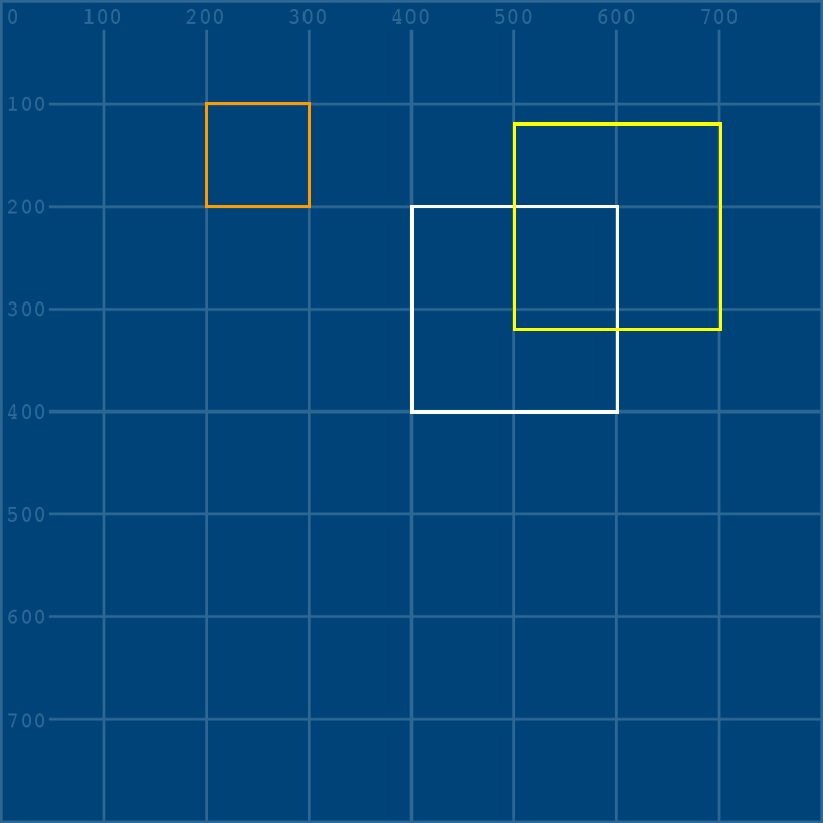
[\begin{matrix} x \\ y \end{matrix}] \times [\begin{matrix} a & b \\ c & d \end{matrix}] = [\begin{matrix} (x \cdot a) + (y \cdot b) \\ (x \cdot c) + (y \cdot d) \end{matrix}]

To perform a scale, value a multiplies the width, and value d multiplies the height. To half the square’s width and height, use a matrix where both a and d are equal to 0.5:

[\begin{matrix} 400 \\ 200 \end{matrix}] \times [\begin{matrix} 0.5 & 0 \\ 0 & 0.5 \end{matrix}] = [\begin{matrix} (400 \times 0.5) + (200 \times 0) \\ (400 \times 0) + (200 \times 0.5) \end{matrix}]

Add some code that draws a new orange square half the size of the white one:

a = 0.5; b = 0
c = 0; d = 0.5
stroke('#FF9900')
quad(
  x*a + y*b,         x*c + y*d,
  x*a + (y+h)*b,     x*c + (y+h)*d,
  (x+w)*a + (y+h)*b, (x+w)*c + (y+h)*d,
  (x+w)*a + y*b,     (x+w)*c + y*d
)

Run the sketch. The orange square is half the size of the white square, but the position has also changed:

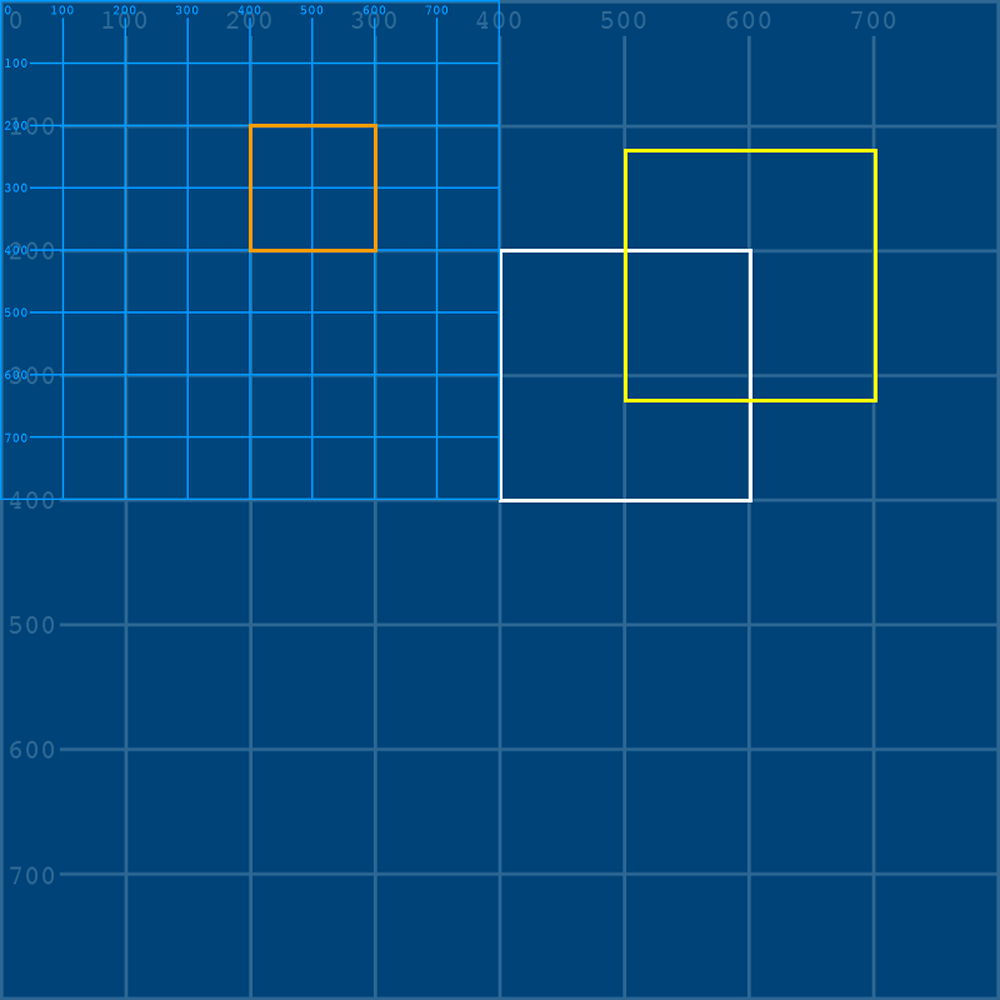
To reveal why the position changes, add the grid-overlay.png file to your code – but halve its size using a third and fourth image() argument:

...

grido = loadImage('grid-overlay.png')
image(grido, 0,0, 800/2,800/2)

a = 0.5; b = 0
c = 0; d = 0.5
stroke('#FF9900')
quad(
  x*a + y*b,         x*c + y*d,
  x*a + (y+h)*b,     x*c + (y+h)*d,
  (x+w)*a + (y+h)*b, (x+w)*c + (y+h)*d,
  (x+w)*a + y*b,     (x+w)*c + y*d
)

As evidenced by the grid overlay, when one performs a scale transformation, the entire grid upon which the shape is plotted scales toward the origin (0,0).

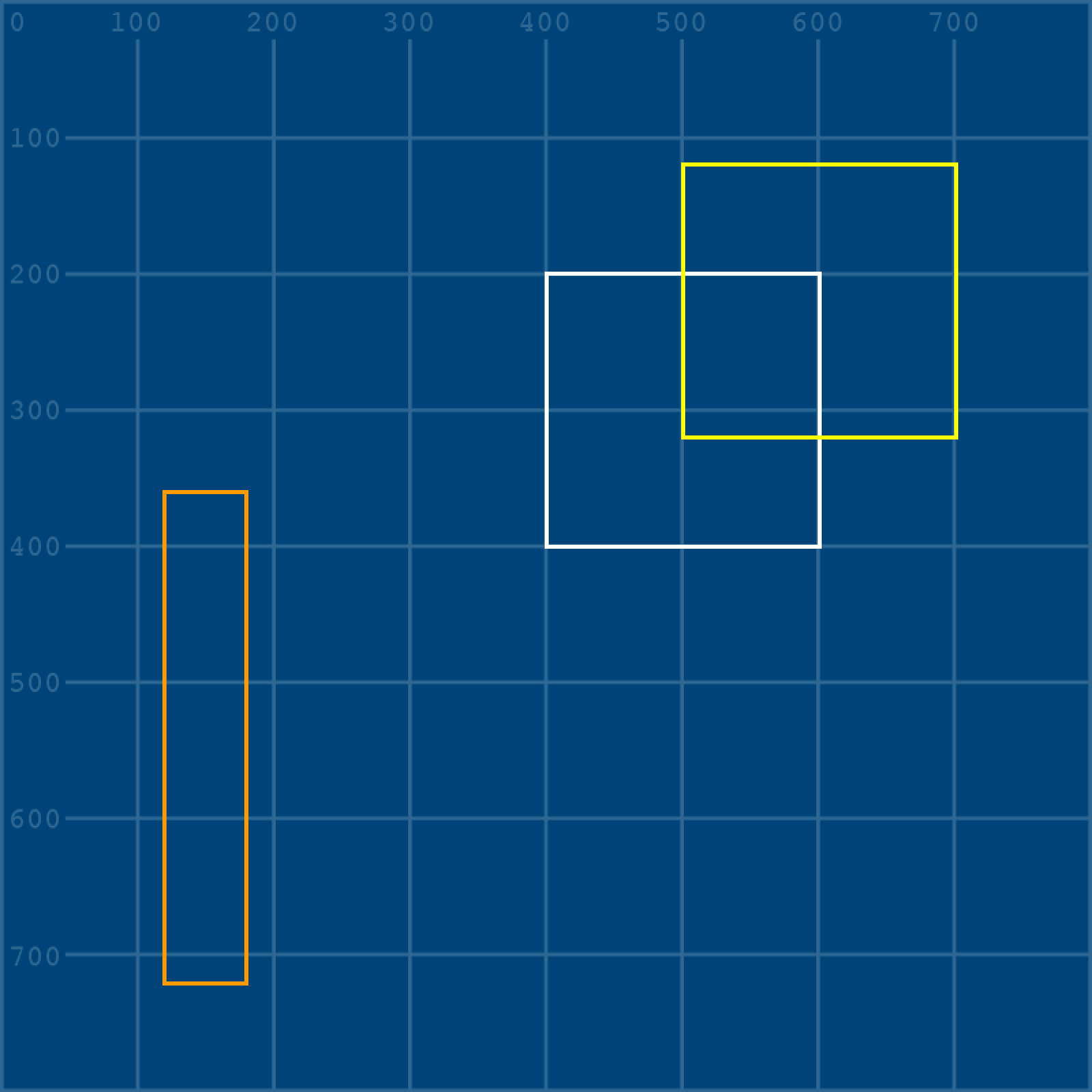
The brighter blue lines and numbers are those of the grid-overlay.png file.

Scaling need not be proportionate. Comment out the grid-overlay image, and adjust your a and b variables for a distorted square:

grido = loadImage('grid-overlay.png')
#image(grido, 0,0, 800/2,800/2)

a = 0.3; b = 0
c = 0;   d = 1.8
stroke('#FF9900')
quad(
  x*a + y*b,         x*c + y*d,
  x*a + (y+h)*b,     x*c + (y+h)*d,
  (x+w)*a + (y+h)*b, (x+w)*c + (y+h)*d,
  (x+w)*a + y*b,     (x+w)*c + y*d
)

Expressed in matrix notation, this is:

[\begin{matrix} 400 \\ 200 \end{matrix}] \times [\begin{matrix} 0.3 & 0 \\ 0 & 1.8 \end{matrix}] = [\begin{matrix} (400 \times 0.3) + (200 \times 0) \\ (400 \times 0) + (200 \times 1.8) \end{matrix}]

Reflect

Reflecting a shape is a matter of scaling one axis by a negative value; then multiplying the other by 1.

For a horizontal reflection use:

[\begin{matrix} x \\ y \end{matrix}] \times [\begin{matrix} - a & 0 \\ 0 & 1 \end{matrix}]

And for a vertical reflection:

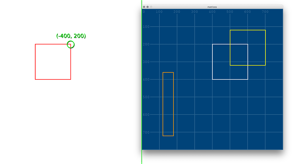
[\begin{matrix} x \\ y \end{matrix}] \times [\begin{matrix} 1 & 0 \\ 0 & - d \end{matrix}]

Be aware, though: reflection operations are relative to the origin (0,0). As an example, add a new red square that’s a horizontal reflection of the white original:

a = -1; b = 0
c = 0;  d = 1
stroke('#FF0000')
quad(
  x*a + y*b,         x*c + y*d,
  x*a + (y+h)*b,     x*c + (y+h)*d,
  (x+w)*a + (y+h)*b, (x+w)*c + (y+h)*d,
  (x+w)*a + y*b,     (x+w)*c + y*d
)

Expressed in matrix notation, this is:

[\begin{matrix} 400 \\ 200 \end{matrix}] \times [\begin{matrix} -1 & 0 \\ 0 & 1 \end{matrix}] = [\begin{matrix} (400 \times -1) + (200 \times 0) \\ (400 \times 0) + (200 \times 1) \end{matrix}]

The result is a square with a width of -200, drawn from a starting coordinate of (-400,200). As this lies beyond left-edge of the display window, it cannot be seen.

The green line indicates the axis of horizontal reflection.

Rotate

Rotation transformations require the trigonometric functions cos() and sin(). Recall, though, that Processing deals in radians rather than degrees, so any arguments you pass these functions must be expressed in radians.

Add a pink version of the white square, rotated 45 degrees (roughly 0.785 radians).

a = cos(0.785); b = -sin(0.785)
c = sin(0.785); d = cos(0.785)
stroke('#FF99FF')
quad(
  x*a + y*b,         x*c + y*d,
  x*a + (y+h)*b,     x*c + (y+h)*d,
  (x+w)*a + (y+h)*b, (x+w)*c + (y+h)*d,
  (x+w)*a + y*b,     (x+w)*c + y*d
)

Expressed in matrix notation, this is:

[\begin{matrix} 400 \\ 200 \end{matrix}] \times [\begin{matrix} cos(0.785) & -sin(0.785) \\ sin(0.785) & cos(0.785) \end{matrix}]

The result is a ‘top-left’ coordinate of roughly (141, 424).

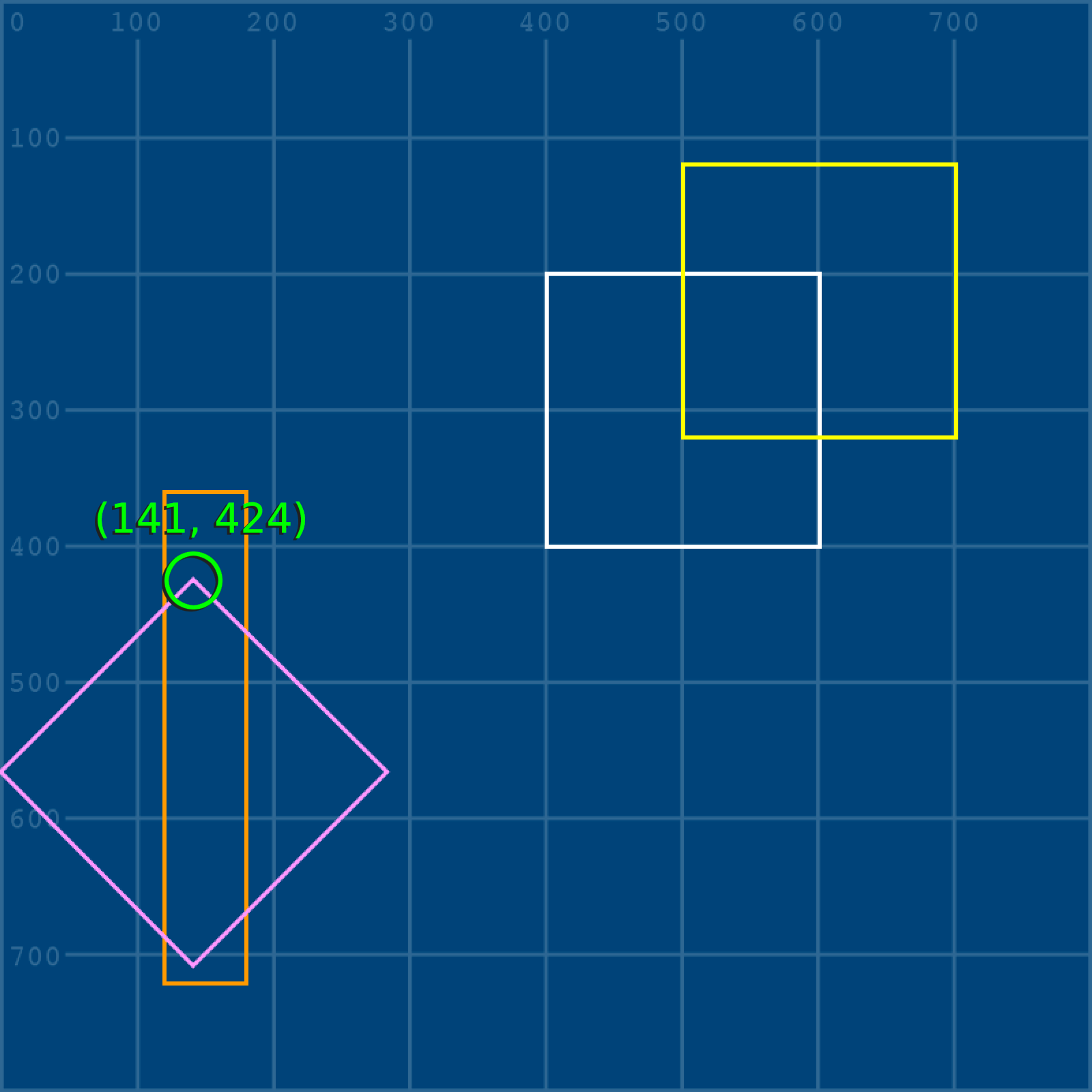
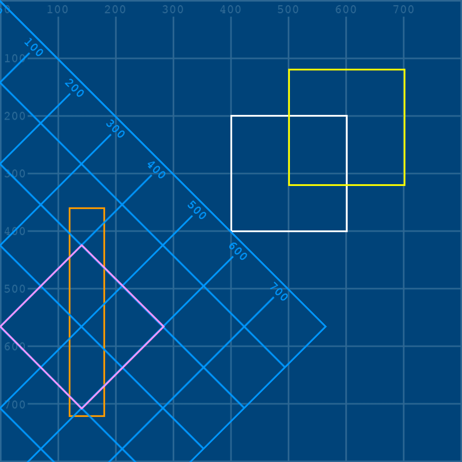
[\begin{matrix} 282.96 + -141.37 \\ 282.73 + 141.47 \end{matrix}] = [\begin{matrix} 141.58 \\ 424.2 \end{matrix}]

With the square rotated 45 degrees, the top-left corner appears in a top-centre position.

As with the other transformations, the axis runs through (0,0). To better visualise this, here’s the rotation represented with a grid-overlay graphic:

Shear

Shearing a shape slants/skews it along the horizontal or vertical axis. The area (or volume), however, remains constant.

To shear horizontally, use:

[\begin{matrix} x \\ y \end{matrix}] \times [\begin{matrix} 1 & b \\ 0 & 1 \end{matrix}]

And for a vertical shear:

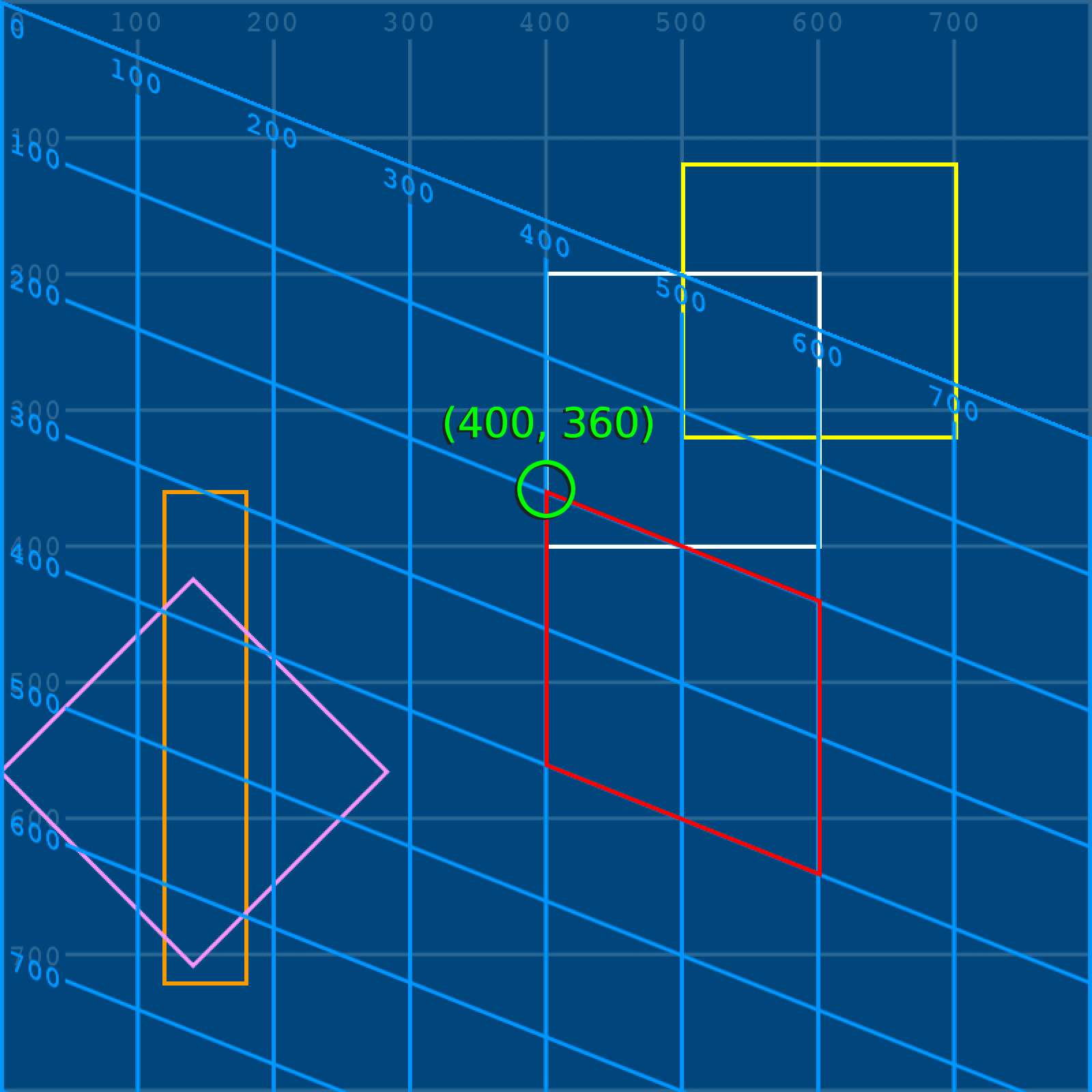
[\begin{matrix} x \\ y \end{matrix}] \times [\begin{matrix} 1 & 0 \\ c & 1 \end{matrix}]

Add a red version of the white square, sheared vertically using a coefficient of 0.4.

a = 1;   b = 0
c = 0.4; d = 1
stroke('#FF0000')
quad(
  x*a + y*b,         x*c + y*d,
  x*a + (y+h)*b,     x*c + (y+h)*d,
  (x+w)*a + (y+h)*b, (x+w)*c + (y+h)*d,
  (x+w)*a + y*b,     (x+w)*c + y*d
)

Expressed in matrix notation, this is:

[\begin{matrix} 400 \\ 200 \end{matrix}] \times [\begin{matrix} 1 & 0 \\ 0.4 & 1 \end{matrix}] = [\begin{matrix} (400 \times 1) + (200 \times 0) \\ (400 \times 0.4) + (200 \times 1) \end{matrix}]

Below is the result, along with a grid-overlay and x-y coordinate label:

This section has introduced some fundamental transformation concepts using matrices while avoiding anything larger than 2 × 2 matrix. If you want to handle larger matrices, take a look at Python’s NumPy library.

^{In programming, a library is a collection of prewritten code. Instead of you having to write everything from scratch, Python provides a system for utilising packages of other people’s code. We’ll be leveraging a few different libraries in these lessons.}

Next up: performing all of the above transformations without having to worry about the math!

Processing Transform Functions

After having done transformations the hard way, grasping Processing’s transform functions is a breeze.

Create a new sketch and save it as “transform_functions”. Within the sketch’s folder, create a “data” subfolder containing a copy of the grid.png and grid-overlay.png files:

grid.png
grid-overlay.png

Add the following setup code (note that grid-overlay.png is loaded but not drawn):

size(800,800)
noFill()
stroke('#FFFFFF')
strokeWeight(3)
grid = loadImage('grid.png')
image(grid, 0,0)
grido = loadImage('grid-overlay.png')

Add a white rectangle, drawn in the same position as that of the last sketch. Because you’ll be using Processing’s built-in transform functions, a rect() will work fine, i.e. there’s no need to use a quad() unless you prefer to.

x = 400; y = 200
w = 200; h = 200
rect(x,y, w,h)

Add a translate(100,-80) function and a duplicate rect() in yellow:

...
x = 400; y = 200
w = 200; h = 200
rect(x,y, w,h)

translate(100,-80)
stroke('#FFFF00')
rect(x,y, w,h)

Add a square, 100 × 100 pixels in width/height, with an x-y coordinate of zero:

...
stroke('#FF0000')
rect(0,0, 100,100)

Run the sketch. The red square can be seen cut-off near the top-left of the display window. The shapes do not change position – rather it’s the coordinate system that does. To better visualise this behaviour, draw the grid-overlay.png after the translate() function:

...
x = 400; y = 200
w = 200; h = 200
rect(x,y, w,h)

translate(100,-80)
image(grido, 0,0)
stroke('#FFFF00')
rect(x,y, w,h)
stroke('#FF0000')
rect(0,0, 100,100)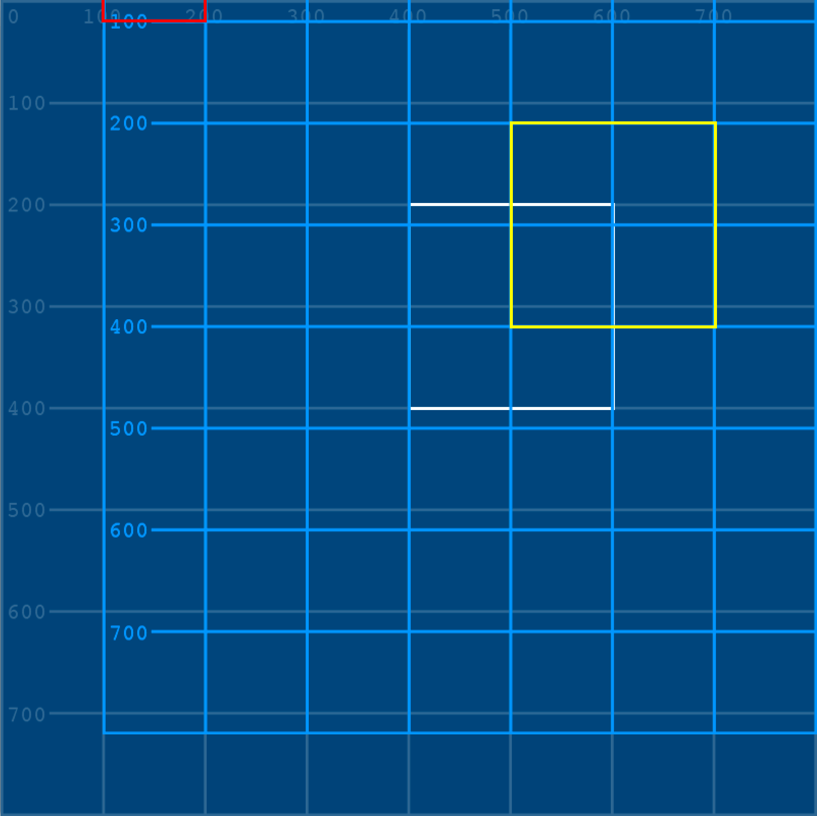

To return the red square to the top-left corner, one could add a translate(-100,80) to offset the prior one – or better yet, isolate the translation. Wrap the translate, image, and yellow square code in a pushMatrix() and popMatrix() function. These will create a new matrix stack within which only the nested shapes (a yellow square, for now) are translated:

...
x = 400; y = 200
w = 200; h = 200
rect(x,y, w,h)

pushMatrix()
translate(100,-80)
image(grido, 0,0)
stroke('#FFFF00')
rect(x,y, w,h)
popMatrix()

stroke('#FF0000')
rect(0,0, 100,100)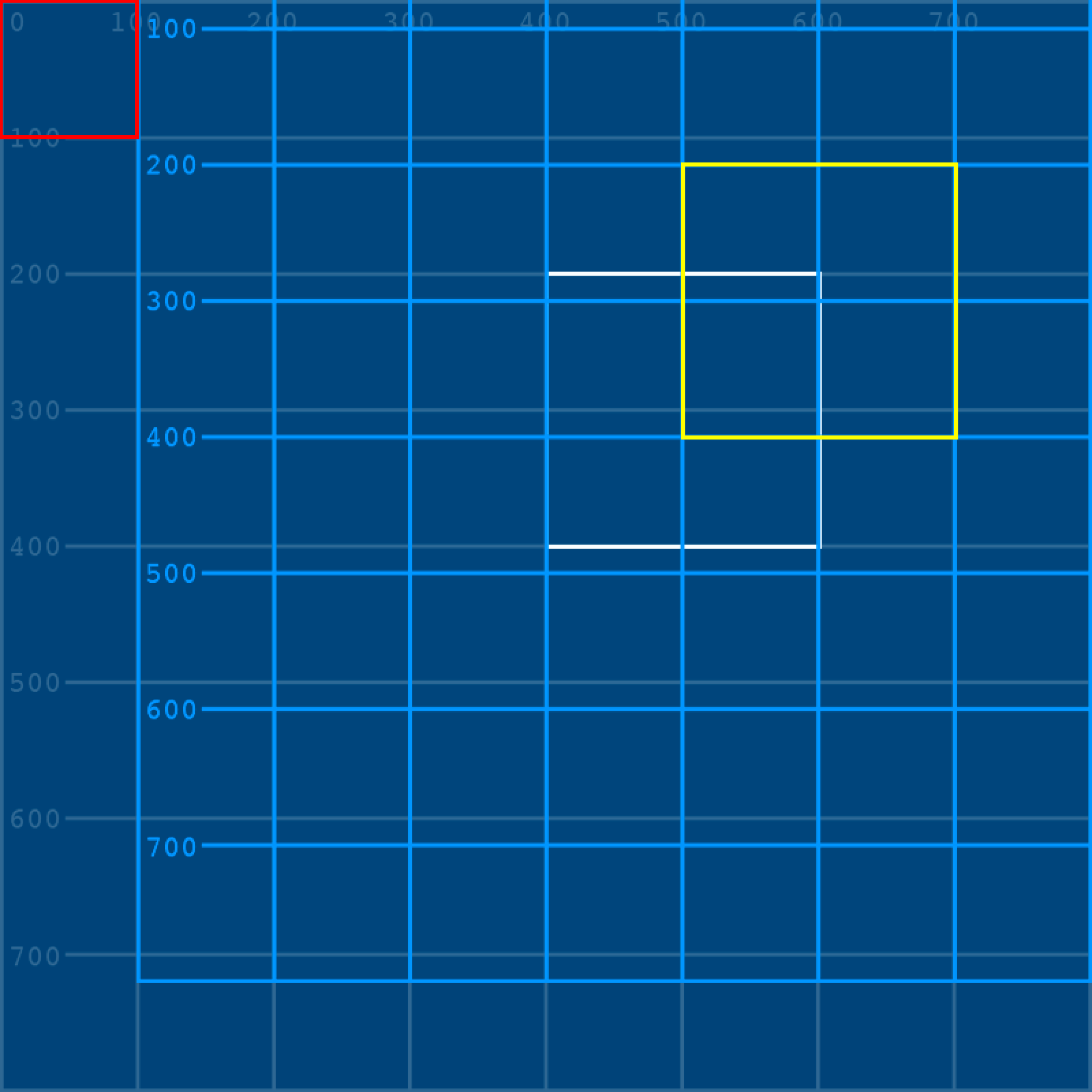

This makes for a useful drawing approach – moving the coordinate system to avoid keeping track using variables, then adding a popMatrix() to return to the original coordinate system. It ultimately depends on what works best for what you are drawing.

In addition to translate(), Processing’s 2D transform functions include, rotate(), scale(), shearX(), and shearY().

What is more, you may combine these as you wish. Add further transform functions to the existing matrix stack:

pushMatrix()
translate(100,-80)
rotate(0.785)
shearY(0.4)
image(grido, 0,0)
stroke('#FFFF00')
rect(x,y, w,h)
popMatrix()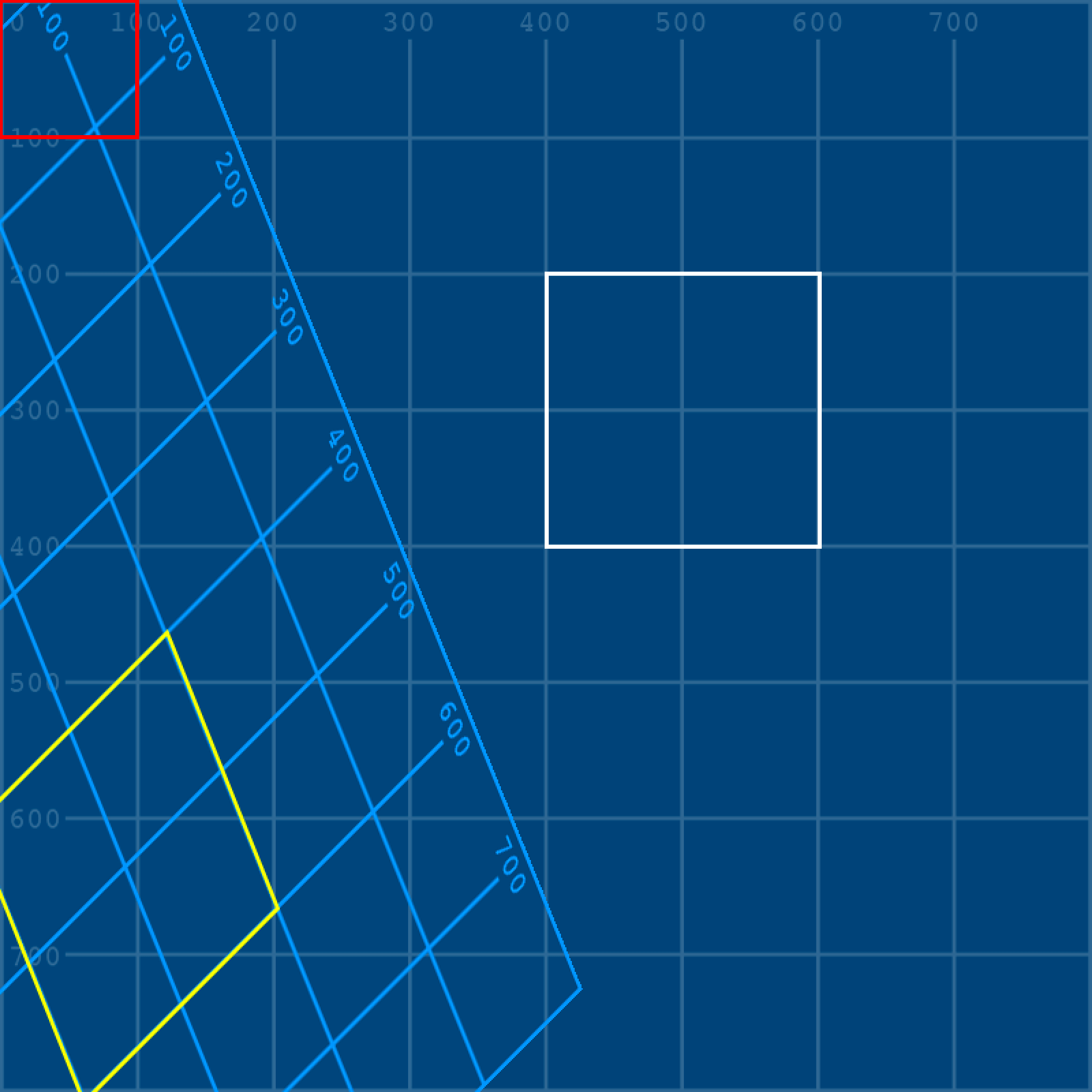

You’ll be using a mix of coordinate tracking and transformation techniques in the tasks to come.

4.3: Time and Date »
Complete list of Processing.py lessons