« 4.2: Transformations |
4.4: Animated Trigonometry »
Time and Date
There are twenty-four hours in a day. But why is this not ten, twenty, a hundred, or some other more ‘rounded’ number? To make things more confusing, these twenty-four hours are then split into twelve AM and twelve PM hours. To understand why this is, one must look back to where the system first originated – around Mesopotamia and Ancient Egypt, circa 1500 BC. These civilisations relied on sundials and water-clocks for day- and night-time timekeeping, which explains the need for the two (AM/PM) cycles. The twelve figure arises from an ancient finger-counting system, where one uses the thumb to count up to twelve on the three bones of each finger.

Not only does this explain the origins of the 12-hour clock, but also the dozen grouping system. Twelve also happens to have the most divisors of any number below eighteen.
If the twelve-hour clocks make time tricky to deal with, time zones only complicate matters further. Given that the earth is a spinning ball circling the sun, it’s always noon along some longitudinal arc of the planet’s surface. Because the earth must rotate a full 360 degrees to complete one day, ‘noon’ moves across the planet’s surface at 15 degrees (360 ÷ 24) each hour, giving rise to 24 solar time zones. But whether or not your watch reads 12:00 depends on the local time zone in which you find yourself. For example, Australia has three such local time zones whereas China has one, despite the latter straddling four solar time zones.
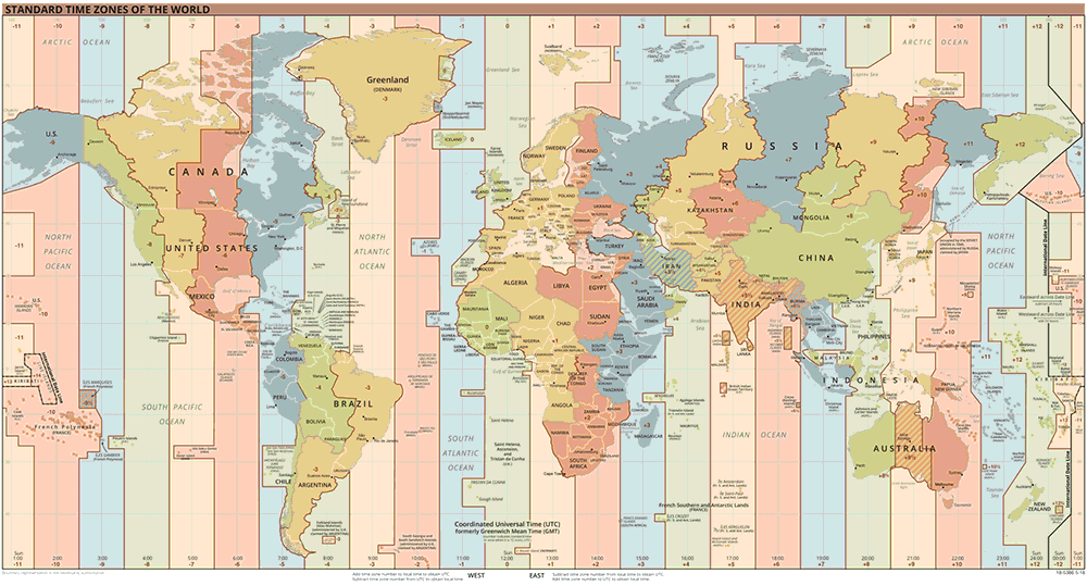
TimeZonesBoy [Public domain], via Wikimedia Commons
Then there are day-light savings hours to contend with (where one day in each year must be 23 hours long; and another, 25). Never mind that each year is comprised of 52 weeks, 12 months (of varying lengths), 365 days … oh, and what about leap years? All of these factors make handling time a complicated task – but, fortunately, Processing provides a number of functions that perform the tricky calculations for you.
Firstly, though, an introduction to UTC (Coordinated Universal Time) will help make time zones more manageable. UTC – which is interchangeable with GMT – lies on zero degrees longitude and is never adjusted for daylight savings. Local time zones can be expressed using a UTC offset, for example:
| China: | UTC+08:00 |
| India: | UTC+05:30 |
| Uruguay: | UTC-03:00 |
The Python datetime library provides a utcnow() method for retrieving UTC timestamps:
import datetime
timestamp = datetime.datetime.utcnow()
# 2018-08-06 07:57:22.817889
Unix timestamps represent the number of seconds that have elapsed since 00:00:00, January 1st, 1970 (UTC):
import time
timestamp = time.time()
# 1533715946.817889
The datetime and time libraries include a complete set of functions for manipulating and managing time data, and depending on what you wish to accomplish you may elect one toolset over the other. However, Processing’s built-in functions that may prove easier to use.
Processing Date and Time Functions
To begin exploring Processing time and date functions, create a new sketch and save it as “date_and_time”. Add the following code:
y = year()
m = month()
d = day()
print('{}-{}-{}'.format(y,m,d))

h = hour()
m = minute()
s = second()
print('{}:{}:{}'.format(h,m,s))
The date and time functions above communicate with your computer clock (local time). Each function returns an integer value, as your Console output will confirm. The string interpolation approach cuts-out the need for multiple + operators, replacing each pair of {} braces with its respective .format() argument.
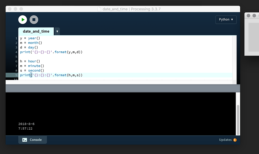
2018-8-67:57:22
Unlike the functions above, millis() does not fetch date and time values from your clock – but instead returns the number of milliseconds (thousands of a second) that have elapsed since starting the program. Add the following code:
ms = millis()
print(ms)
Run this code. The ms value is unlikely to exceed 700. However, the number of milliseconds printed to Console will vary depending on any code executed prior to the millis() function call. For example, add a for loop and have it draw a million squares:
...

for i in range(1000000):
    rect(10,10,10,10)

ms = millis()
print(ms)
The ms value is now likely to exceed 1000. I say “likely”, because your computer specs and any processes running in the background will have an influence. As a case in point, running this code on my laptop while transcoding a video file added around another thousand milliseconds to the readout.
The millis() function operates independently of frame rate (which is prone to fluctuation). To monitor how many frames have elapsed, use the frameCount system variable.
Sprite Sheet Animation
A sprite is a single graphic comprised of pixels. Multiple sprites can be combined to create a scene like that of this Mario Bros. level:
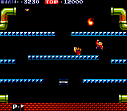
Nintendo Co., Ltd. [Copyright], from Wikipedia
Study the screenshot above; notice how the blue bricks are all clones of one another. Rather than place a unified environment image into the scene, the developer repeats a single blue brick at the positions necessary to form the platforms. The paved red surface is also formed using a repeating tile. Mario, the turtle, and the fireball are also sprites, although, unlike the environmental sprites, these are animated. Every frame that comprises Mario’s walk-cycle is packed into a single sprite sheet – like in this Nyan Cat example:
PRguitarman [Standard YouTube License / redrawn as 6-frame sprite sheet], from Youtube
By packing every frame into a single image, the developer need only load a single sprite sheet graphic, thus reducing memory and processing overhead. Additionally, all of the background elements are packed into a separate sprite sheet of their own. The technique dates back to early video game development but has since been utilised in other domains, such as web development.
To create a sprite sheet animation of your own, create a new sketch and save it as “spritesheet_animation”. Within this, create a “data” folder. Download a copy of the Nyan Cat sprite sheet and place it in the data folder:
Add the following code:
def setup():
    size(300,138)
    frameRate(12)

def draw():
    background('#004477')
    nyan = loadImage('nyancat-spritesheet.gif')
    xpos = 0
    image(nyan, xpos,0)
A sprite sheet must move about within a containing box, as if behind a sort of mask. In this instance, the display window will serve as that ‘mask’. The nyancat-spritesheet.gif is 1500 pixels wide and 138 pixels high. This means that each frame is 300 pixels wide (1500 ÷ 5), hence the size(300,138) line. To advance a frame, the nyancat-spritesheet.gif graphic needs to be shifted 300 pixels further left with each iteration of draw(). The position can be controlled using frameCount, but combined with a modulo operation to bring it back to zero every fifth frame:
def setup():
    size(300,138)
    frameRate(12)

def draw():
    background('#004477')
    nyan = loadImage('nyancat-spritesheet.gif')
    xpos = (frameCount % 5) * 300 * -1
    image(nyan, xpos,0)
Run the sketch to verify that Nyan Cat loops seamlessly.
This was an elementary introduction to sprite sheets. It’s hardly an ideal approach (that modulo operation only grows more demanding as the frameCount increases). Most sprite sheets are grid-like in appearance, with graphics arranged in rows and columns. Should you wish to create 2D game – using Processing or another platform – you’ll want to research this topic further.
4.4: Animated Trigonometry »
Complete list of Processing.py lessons