« 4.3: Time and Date |
5.1: Lists »
Animated Trigonometry
It’s assumed that you possess some (if only a very little bit of) trigonometry knowledge. What follows is a practical and visual introduction to trigonometry in motion. Clock, metronome, and piston mechanisms all exhibit elegant rhythms that can be reproduced using sine and cosine functions.
Analogue Clock Task
Trigonometry focuses on triangles but is also associated with circles. A refresher on radians is required before venturing further, and what better way to link angles and circles than analogue clocks?
Creating a digital clock in Processing is a simple matter of combining time and text functions. For an analogue clock, however, one must convert the hours, minutes, and seconds into angles of rotation.
Create a new sketch and save it as “analogue_clock”. To help you along, begin with some code that prints out Processing’s pi constants:
print(PI)
print(TWO_PI)
print(TAU)
print(HALF_PI)
print(QUARTER_PI)
These will prove handy for programming your clock. For instance, rather than entering PI/2 each time you want to rotate something 90 degrees, you can instead use HALF_PI. Regarding TAU … well, there’s this big, nerdy mathematician war raging over whether it’s better to use pi or tau. Basically, π represents only half a circle in radians, so 2π tends to spring up in formulae all over the place, i.e. there are 2π radians in a circle. In 2001 it was proposed that a new constant be devised to represent a full circle; in 2010 it was decided that this value would be represented using the tau symbol (τ). The table below represents equivalent expressions using TAU and PI constants, additionally listing their approximate decimal values:
TAU |
` = ` |
TWO_PI |
` = ` |
6.284 |
TAU/2 |
` = ` |
PI |
` = ` |
3.142 |
TAU/4 |
` = ` |
HALF_PI |
` = ` |
1.571 |
TAU/8 |
` = ` |
QUARTER_PI |
` = ` |
0.785 |
To begin the clock, draw the face and hour hand:
...

def setup():
    size(600,600)
    noFill()
    stroke('#FFFFFF')

def draw():
    background('#004477')
    translate(width/2, height/2)
    strokeWeight(3)
    ellipse(0,0, 350,350)

    strokeWeight(10)
    line(0,0, 100,0)
The hour hand currently rests along zero radians (pointing East). Recall that when drawing arcs, the angle opens clockwise (southward). However, our clock will be offset by three hours should the hand begin from a 3 o’clock position. Correct this using a rotate() function:
    ...

    rotate(-HALF_PI)

    strokeWeight(10)
    line(0,0, 100,0)
The next step is to calculate how many radians the hand advances with each hour. Consider that a complete rotation is tau radians; therefore one hour equals tau over __? Multiply this by the hour() function and use a push/popMatrix to perform the rotation. Once the hour hand is functional, add the minute and second hands. Your finished clock will look something like this:

With a good grasp of radians, we can move onto trigonometric functions. Should you ever need to convert between radians and degrees, look up the radians() and degrees() functions.
SOH-CAH-TOA
Remember SOHCAHTOA (sounded out phonetically as sock-uh-toe-uh)? That mnemonic device to help you remember the sine, cosine, and tangent ratios? Remember how you thought you’d never use it again after leaving school? To refresh your memory, the acronym stands for:
| sine | ` = ` |
opposite ÷ hypotenuse |
| cosine | ` = ` |
adjacent ÷ hypotenuse |
| tangent | ` = ` |
opposite ÷ adjacent |

TheOtherJesse [Public domain], from Wikimedia Commons
Remember unit circles? A unit circle is a circle with a radius of one:

In the above illustration, angle theta (θ) is equal to 45 degrees – or roughly 0.785 radians – or to be more accurate, pi over 4, which may be expressed as QUARTER_PI in Processing. We’ll return to the unit circle in a moment. For now, create a new sketch and save it as “sohcahtoa”. Add the following code:
theta = 0
radius = 1
s = 200 # scale variable
def setup():
size(600,600)
noFill()
stroke('#FFFFFF')
strokeWeight(3)
def draw():
global theta
background('#004477')
translate(width/2, height/2)
diameter = radius*s*2
ellipse(0,0, diameter,diameter)
x = cos(theta)
y = sin(theta)
print(
round(x,1),
round(y,1)
)
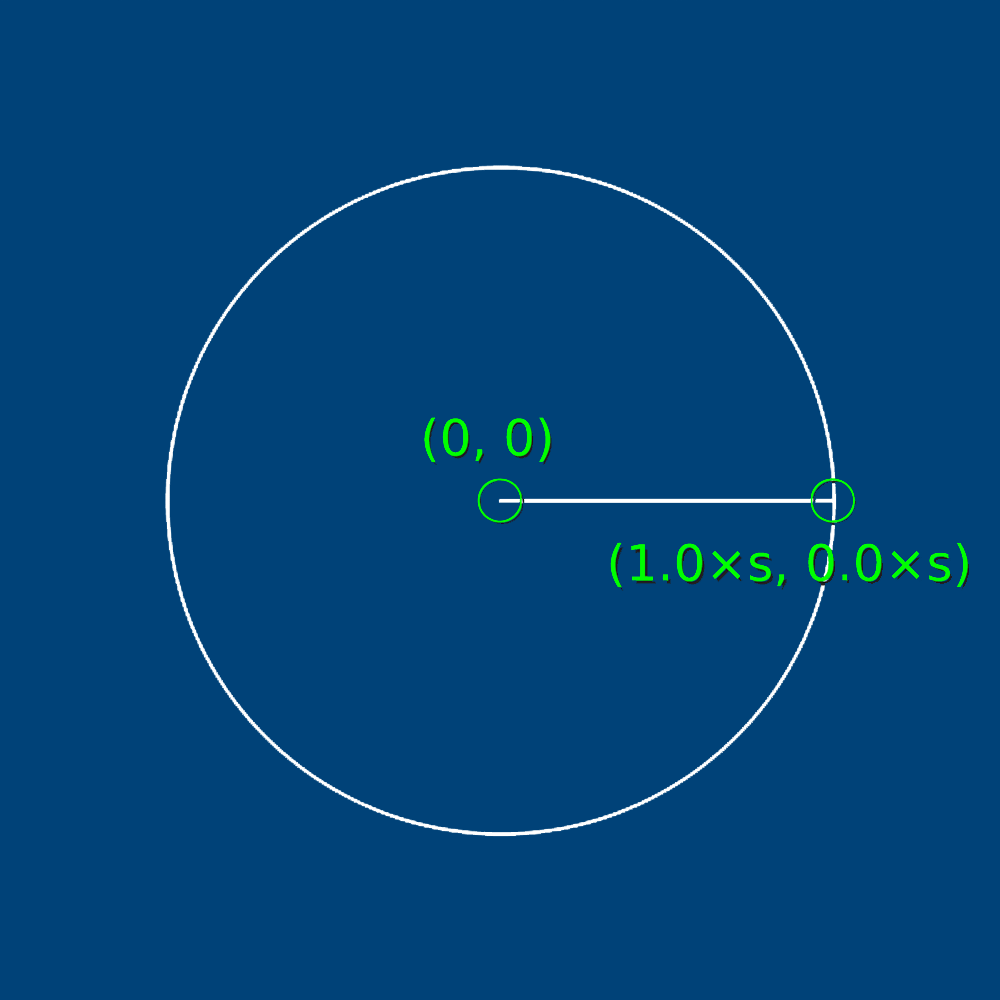
line(0, 0, x*s, y*s)A unit circle would be far too small to work with, hence the inclusion of an s variable for scale. Rather than dealing with a radius of 1, we now have a circle with a radius of 200. Provided all coordinates are scaled by the same factor, the trigonometry calculations will work fine. Run the code. The Console will display lines of (0.0, 1.0) pairs. To avoid printing lengthy floating-point values, these have been rounded to one decimal place. Within the line() function’s arguments, x and y are scaled by s – an integer of 200 – to calculate the line’s endpoint:
Increase the angle slightly, then run the code to see what happens:
    theta = 0.1
    ...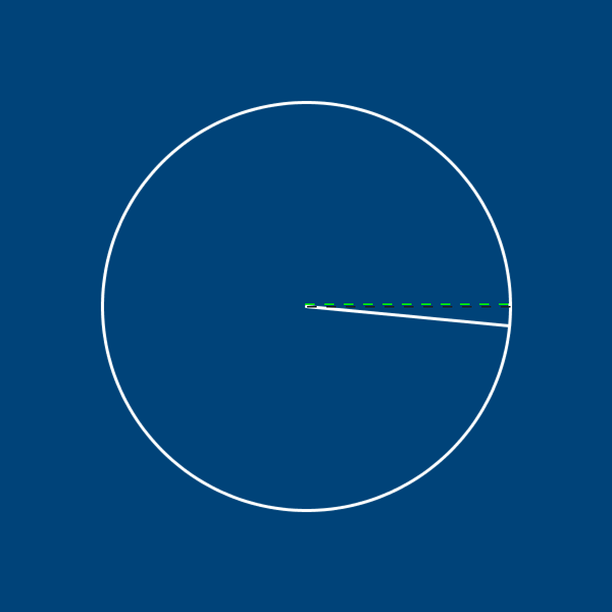
The angle opens in a clockwise direction. To reverse this, multiply the y-coordinate by negative one. To further mimic the unit circle illustration, set the theta variable to 45 degrees (using radians, of course).
theta = QUARTER_PI
...

def draw():
    ...
    line(0, 0, x*s, y*s*-1)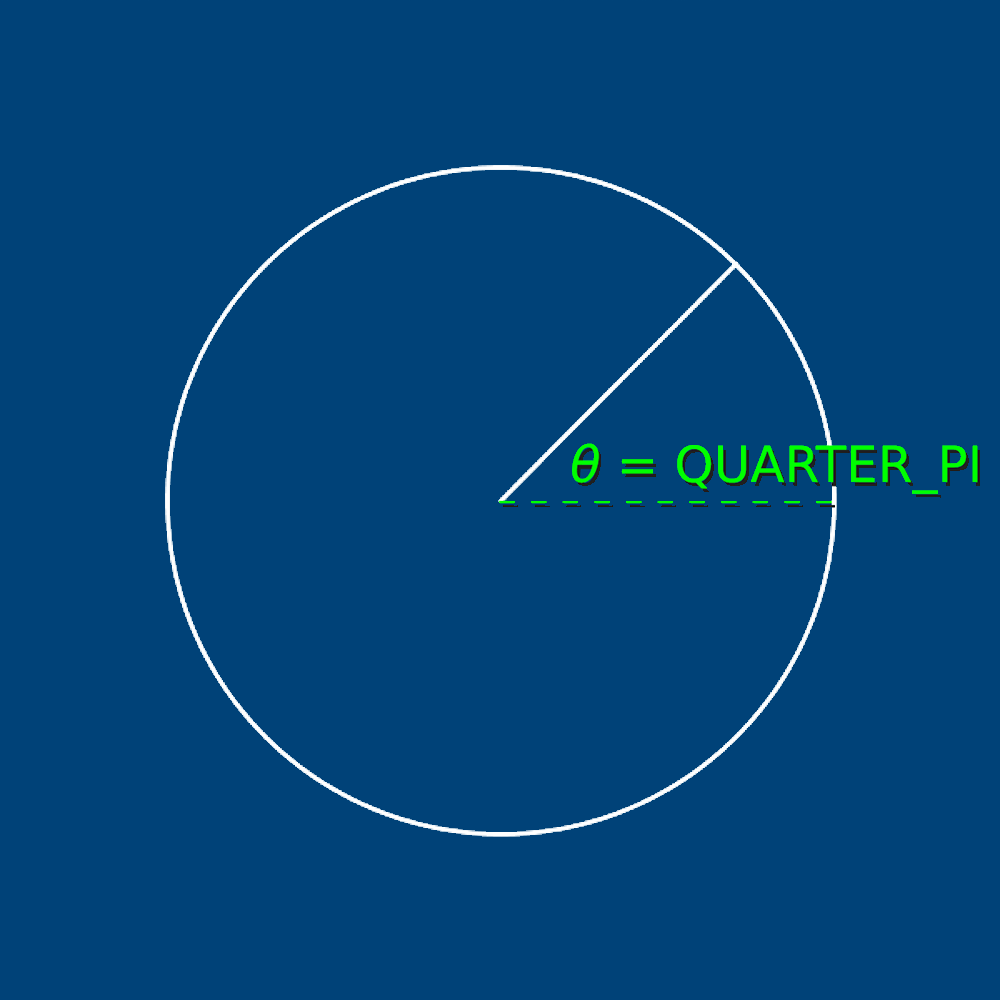
From the Console output, one can see that sin θ returns a value of 0.7, as does cos θ. Therefore, where theta equals QUARTER_PI, sin and cos are equal – but these values drift apart as you increase/decrease the angle. The concept can be illustrated using a unit circle:

To understand how this all works, click the image below and watch the cool animation for about ten seconds.
LucasVB [Public domain], from Wikimedia Commons
The frame below captures the moment where θ reaches 45 degrees (QUARTER_PI radians).
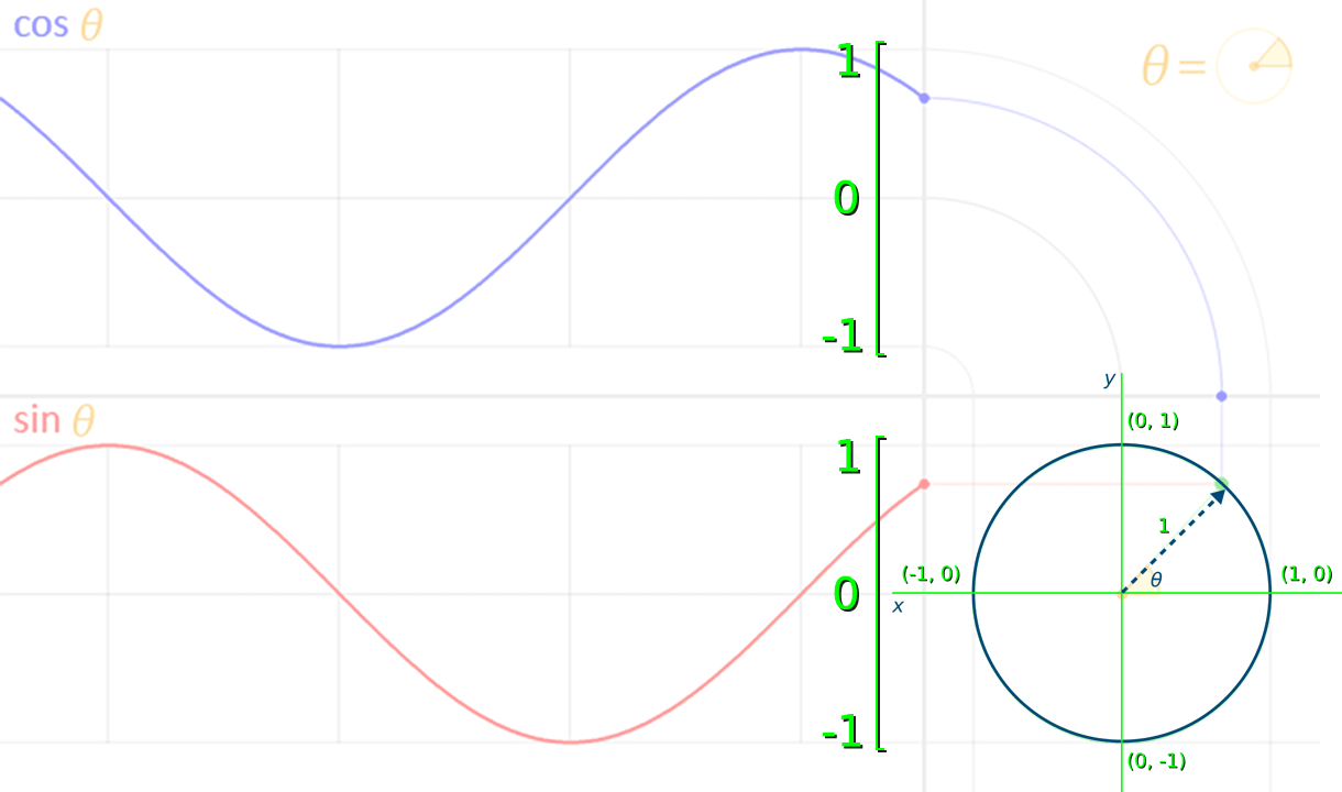
The value for sin θ – the red dot at the end of the red wave – is equal to roughly 0.7. Take note of how the sine function returns values between 1 and -1 that indicate the y-coordinate of where the arrow touches the circle’s circumference. The blue cos wave also oscillates 1 and -1, representing the arrow tip’s x-coordinate.
Increment theta by 0.05 with each new frame, and a smaller circle to capture the sine wave’s vertical motion:
def draw():
    ...
    ellipse(-width/2+40, y*s*-1, 10, 10)
    theta += 0.05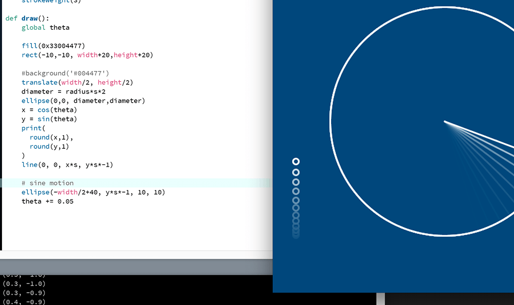
Add another small circle to capture the cosine wave’s horizontal motion:
def draw():
    ...
    ellipse(-width/2+40, y*s*-1, 10, 10)
    ellipse(x*s, -height/2+40, 10, 10)
    theta += 0.05
And, finally, add another small circle at the point where the radius connects to the circumference:
def draw():
    ...
    ellipse(-width/2+40, y*s*-1, 10, 10)
    ellipse(x*s, -height/2+40, 10, 10)
    ellipse(x*s, y*s*-1, 10, 10)
    theta += 0.05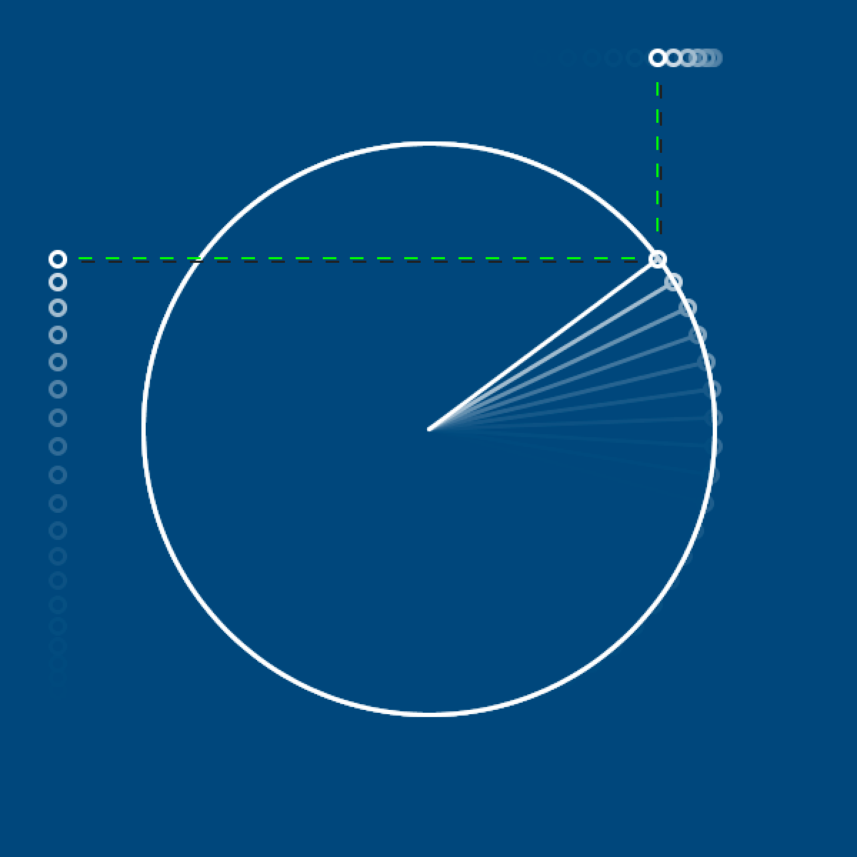
Sine (and cosine) wave patterns are studied in various fields, including physics, engineering, and signal processing.
What about the …-TOA part?
Tangent (tan) functions do not produce wave-like graphs. Perhaps one of the neatest practical examples of tan is xeyes, albeit an application of tan’s inverse function, arctangent. Since the early days of the Linux X Window System, developers have included a feature that places a pair of eyes somewhere on the desktop to help users locate the mouse cursor. This is especially handy for multi-head arrangements where there’s some distance between displays.
The original uploader was Choas at German Wikipedia. [GPL], via Wikimedia Commons
Processing provides a 2-argument arctangent function called atan2() which can be used to find an angle between two points. To see this in action, create a pair of xeyes of your own by adding the following code to your “sohcahtoa” sketch:
def draw():
    ...

    # left eye
    leftx = 180
    lefty = 255
    leftr = atan2(
      y*s*-1 + lefty*-1,
      x*s + leftx*-1
    )
    pushMatrix()
    translate(leftx,lefty)
    rotate(leftr)
    ellipse(0,0, 40,40)
    ellipse(8,0, 10,10)
    popMatrix()

    # right eye
    rightx = 250
    righty = 255
    rightr = atan2(
      y*s*-1 + righty*-1,
      x*s + rightx*-1
    )
    pushMatrix()
    translate(rightx,righty)
    rotate(rightr)
    ellipse(0,0, 40,40)
    ellipse(8,0, 10,10)
    popMatrix()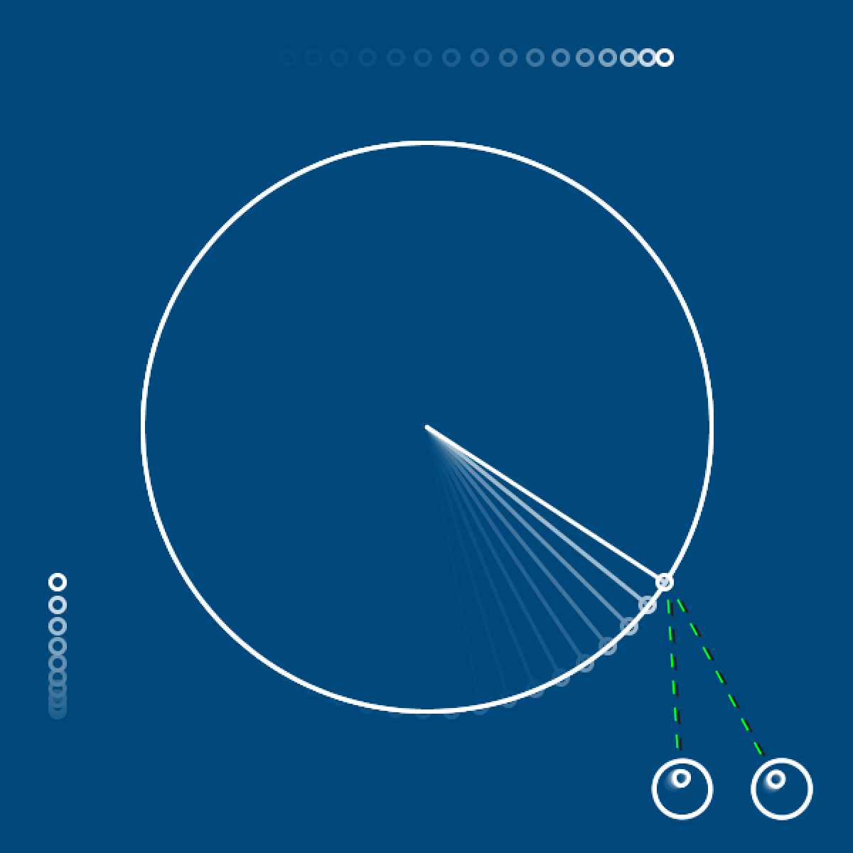
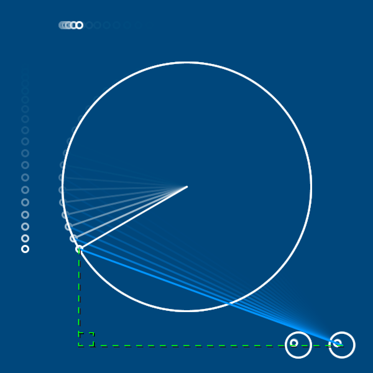
The distance between the x/y-coordinate pair of the target (the small circle at the end of the radius line) and the origin (an eye) indicate the lengths of the opposite and adjacent sides of a right-angled triangle. The atan2() function accepts these two distance values:
atan2(y-distance, x-distance)
To help make visual sense of this, program a line connecting the target and the right eye:
    ...

    # hypotenuse
    stroke('#0099FF')
    ydiff = y*s*-1 + righty*-1
    xdiff = x*s + rightx*-1
    line(
      rightx + xdiff, righty + ydiff,
      rightx, righty
    )
    stroke('#FFFFFF')
From here, Processing calculates the ratio between the opposite and adjacent sides. Recall that the tangent is equal to opposite over adjacent (…-TOA). So – whereas the tan function accepts an angle and returns a ratio – it’s inverse, arctangent, accepts the ratio and returns the angle.
If you’ve some trouble wrapping your head around atan2(), then do not fret; the upcoming task requires only sin() and cos() functions.
Engine task
Time for a final challenge before moving onto lesson 5! Recreate the animation below.

Technically speaking, the piston motion in such an engine design is not quite sinusoidal, but very close. If you’d like another engine challenge, perhaps try the perfectly sinusoidal Scotch yoke.
Lesson 5
That’s it for lesson 4. If you’ve made it this far – the next lesson should be a breeze! Lesson 4 was undoubtedly more mathematical than most, and probably longer, too.
You’ve dealt with string, integer, floating-point, and boolean datatypes. In lesson 4, you’ll explore datatypes that hold a collection of elements – namely Python list and dictionary types. If you’ve some programming experience, you may have encountered something similar (arrays) in other languages? If not, do not stress – we’ll begin with the very basics. As this subject matter works nicely with graphs, we’ll also explore interesting to visualise data.
5.1: Lists »
Complete list of Processing.py lessons
References
- http://lostmathlessons.blogspot.com/2016/03/bouncing-dvd-logo.html
- https://commons.wikimedia.org/wiki/File:DVD_logo.svg
- https://en.wikipedia.org/wiki/Beta_movement