Processing.py in Ten Lessons

Randomness

The best a computer can do is simulate randomness. Think about this for a moment: if you request a random number from a computer, it will need to run some non-random set of instructions to pull a value. That said, computers can manage a pretty good job of this, relying on algorithms that generate pseudorandom numbers whose sequential appearance is statistically similar enough to a truly random sequence. This is okay for shuffling through your music collection, but best avoided for gambling and security applications.

For ‘true’ random numbers, computers can rely on things like key-stroke timings. For instance, you may have pressed your last key 684 milliseconds past the tick of the previous second. In the quest for true randomness, researchers have relied on everything from dice to roulette wheels, and between the mid-1920s and 50s one could even purchase special books full of random numbers. If you are really serious about plucking random numbers from the universe, there are hardware devices that rely on various quantum phenomena, like radioactive decay. However, for most applications, pseudorandomness will suffice.

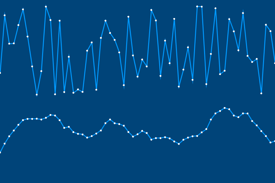
So, what do random sequences look like? First, consider Perlin noise. In 1983, Ken Perlin developed an algorithm for synthesising organic textures and forms – like terrains, fire, smoke, and clouds. The graphs below plot random points (vertical axis) over fixed intervals of time (horizontal axis). The upper line represents a sequence of ‘purely’ random points, whereas the lower line charts values generated with Perlin noise. From this, you can visually appreciate why the ‘smoother’ Perlin noise is better suited for generating something like a mountain range.

Random (top) verse Perlin noise (bottom) sequences.

Processing has functions for Perlin noise, but we’ll focus on the random() and randomSeed() functions.

Random Functions

Create a new sketch and save it as “random_functions”. Add the following setup code:

size(600,600)
background('#004477')
noFill()
stroke('#FFFFFF')
strokeWeight(3)

The random() function takes one or two arguments. One argument defines an upper limit:

...

x = random(5)
print(x)

The above code will display a random floating point value between 0 and 5 (starting at zero and up to, but not including, five). Two arguments represent an upper- and lower-limit respectively:

x = random(5)
print(x)
x = random(5,10)
print(x)

The above displays a random floating point value between 5 and 10. If it’s a random integer you seek, wrap this the x in an int() function. This converts the floating point to an integer by removing the decimal point and everything that follows it (effectively, rounding-down):

x = random(5)
print(x)
x = random(5,10)
print(x)
print( int(x) )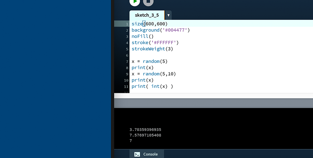

Given that the values are random, the Console output will appear different each time you run the sketch.

The next step is to generate one hundred random values. Rather than print a long list in the Console area, plot them as a series of points along the same y-axis:

...

for i in range(100):
    point( random(width), height/2 )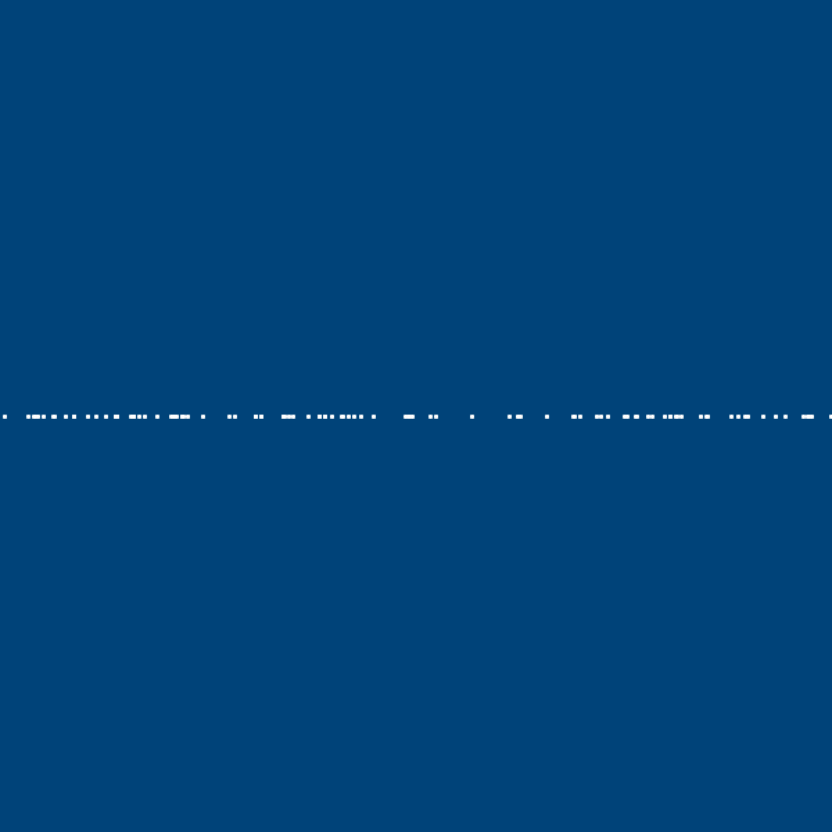

The spread of points will vary each time the sketch is run.

Now edit the loop. Change the range to 1000 and plot the point using both a random x- and y-coordinate:

for i in range(1000):
    point( random(width), random(height) )

Four runs of the same code. Notice (perhaps by comparing a given corner) how each is unique.

Each time the code is run, it produces a slightly different pattern. Recall, though, that these are pseudorandom sequences. What the random() function does is pick an initial random number (based on something such as keystroke timing), then generates an entire sequence based upon this. The initial value is referred to as the seed. Using Processing’s randomSeed() function, one can set the seed parameter manually, thereby ensuring that the same sequence of pseudorandom numbers is generated each time the sketch is run. Add a randomSeed() to your working sketch – the argument may be any integer, but use 213 to verify that your output matches that depicted below.

randomSeed(213)
size(600,600)
...

Unlike the earlier versions in which no random seed had been defined, every run of the code produces the same pattern, on any computer that executes it. This is useful in many applications. As a concrete example, suppose you developed a platform game in which the positions of obstacles are randomly generated. This feature saves you a lot of time, as you no longer have to design each level manually. However, you find that certain sequences of random numbers produce more engaging levels than others. If you are aware of these key seed values, you can reproduce each good level with an integer.

Truchet Tiles

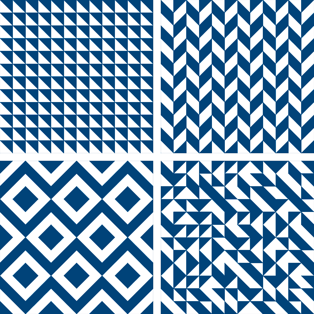
Sébastien Truchet (1657–1729), a French Dominican priest, was active in the fields of mathematics, hydraulics, graphics and typography. Among his many contributions, he developed a scheme for creating interesting patterns using tiles – which have since become known as Truchet tiles. The original Truchet tile is square and divided by a diagonal line between opposing corners. This tile can be rotated in multiples of ninety degrees to produce four variants.

The original Truchet tile, presented in its four possible orientations.

These tiles are arranged on a square grid – either randomly, or according to some pattern – to create aesthetically-pleasing patterns.

Systematic versus random (bottom-right) Truchet tile arrangements.

There are other Truchet tile forms, such as the quarter-circle tile:

Truchet quarter-circle tile presented in its two possible orientations.

Using the looping and randomness techniques from the lesson, you’ll now experiment with this. Create a new sketch and save it as “truchet_tiles”. Add the following setup code, which includes a single tile:

size(600,600)
background('#004477')
noFill()
stroke('#FFFFFF')
strokeWeight(3)

arc(0,0, 50,50, 0,PI/2)
arc(50,50, 50,50, PI,PI+PI/2)

Now comment-out the arc lines and tile the entire display window using a for loop:

#arc(0,0, 50,50, 0,PI/2)
#arc(50,50, 50,50, PI,PI+PI/2)

col = 0
row = 0

for i in range(1,145):
    arc(col,row, 50,50, 0,PI/2)
    arc(col+50,row+50, 50,50, PI,PI+PI/2)
    col += 50

    if i%12 == 0:
        row += 50
        col = 0

The next step is to randomise each tile’s orientation. Because there are only two options, the loop must effectively ‘flip a coin’ with each iteration. A random(2) will return floating point values ranging from 0.0 up to 2.0. Converting the result to an integer, therefore, produces a 0 or 1.

for i in range(1,145):
    print( int(random(2)) )

    arc(col,row, 50,50, 0,PI/2)
    ...

After verifying that the above code prints lines of 1 or 0 to the Console, adapt it to display True/False results.

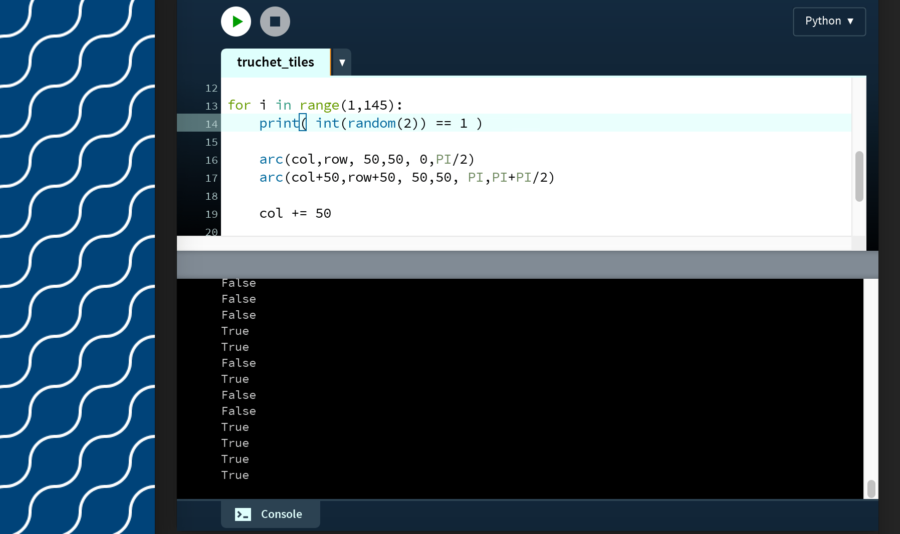
for i in range(1,145):
    print( int(random(2)) == 1 )

    arc(col,row, 50,50, 0,PI/2)
    ...

Because this operation returns a boolean value, it can be used as an if statement condition. Add an if-else structure:

for i in range(1,145):
    #print( int(random(2)) == 1 )

    if int(random(2)) == 1:
        arc(col,row, 50,50, 0,PI/2)
        arc(col+50,row+50, 50,50, PI,PI+PI/2)
    else:
        arc(col+50,row, 50,50, PI/2,PI)
        arc(col,row+50, 50,50, PI+PI/2,2*PI)

    col += 50

    if i%12 == 0:
        row += 50
        col = 0

As your programs grow more complex, you’ll find multiple ways to code the same outcome. For example, you could have laid the quarter-circle Truchet tiles by using a loop within a loop, using range() functions with a step-size argument, in various combinations. See if you can program the randomised quarter-circle sketch using a structure like this:

for row in range(0, height, 50):
    for col in range(0, width, 50):
        ...

If you’ve ever played the strategy game Trax, this pattern will look familiar. Another tile-based strategy game, Tantrix, uses a hexagonal adaption of a Truchet tile.

Tiles are an exciting area to explore using Processing, and we’ll look at other types in the lessons to come.

Progressively-Jittery Quads Task

Here’s the final challenge before moving onto lesson 4.

This one appears in Ira Greenberg’s Processing: Creative Coding and Generative Art in Processing 2 (page 80). It’s a great book that presents a fun and creative approach to learning programming. It’s based on Processing’s Java mode (rather than Python) and well worth a read.

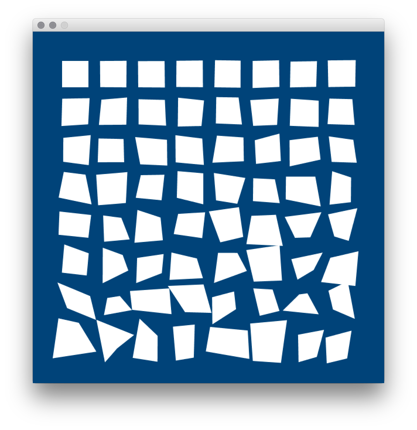
You’ll be referencing this image during the task, so it may be useful to save a copy and open a preview of it alongside your Processing editor.

Create a new sketch and save is “progressively_jittery_quads”. The display window is 600 pixels wide by 600 pixels high. Go ahead and complete the task.

Lesson 4

That’s it for lesson 3. Kudos for getting through it – control flow is a tricky matter to get your head around at first! I trust that introducing random values has inspired some exciting project ideas.

The next lesson deals with animation. There’s a bit you need to know about matrices and trigonometry, though. If you find yourself experiencing disturbing flashbacks of high school math class – take a deep breath and relax. Lesson 4 will be a practical and visual reintroduction to these concepts, with Processing crunching all of the numbers for you.

If statements and loops will reappear throughout this course, which will give you plenty of opportunities to master them. If you’ve some extra time, read up on the continue and break statements. These are two useful loop techniques that allow one to skip over iterations, or to ‘break-out’ of loop structures.

4.1: Animation »
Complete list of Processing.py lessons

References

https://www.apress.com/us/book/9781430244646
https://www.youtube.com/watch?v=SxP30euw3-0

Processing.py in Ten Lessons – 3.4: Randomness