« 6.1: Image Formats |
6.3: Halftones »
Colour Channels
Each pixel on your screen is mixed using three primary colours: red, green, and blue. Another way to think of this is three monochrome images (or channels) that control the levels of each primary, combined into one image.
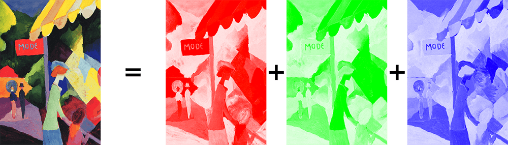
Modefensterseparated into red, green, and blue channels.
Notice how the whiter areas of Modefenster, such as the foreground woman’s face, appear solid for every channel. Recall that, to produce white, the red, green, and blue channels must combine at full intensity.
Sometimes it’s preferable to work with four channels. For instance, you may need an alpha channel for transparency. Another scenario is print design. Colour printers use a four-colour CMYK model: cyan, magenta, yellow, and black. If you’ve ever replaced ink cartridges in your printer, you’ve probably noticed this. For CMYK, desktop publishing file formats can handle 32-bit colour values. For instance, a blue mixed with 100% cyan and 50% appears as:
In hexadecimal notation, it’s:
FF800000
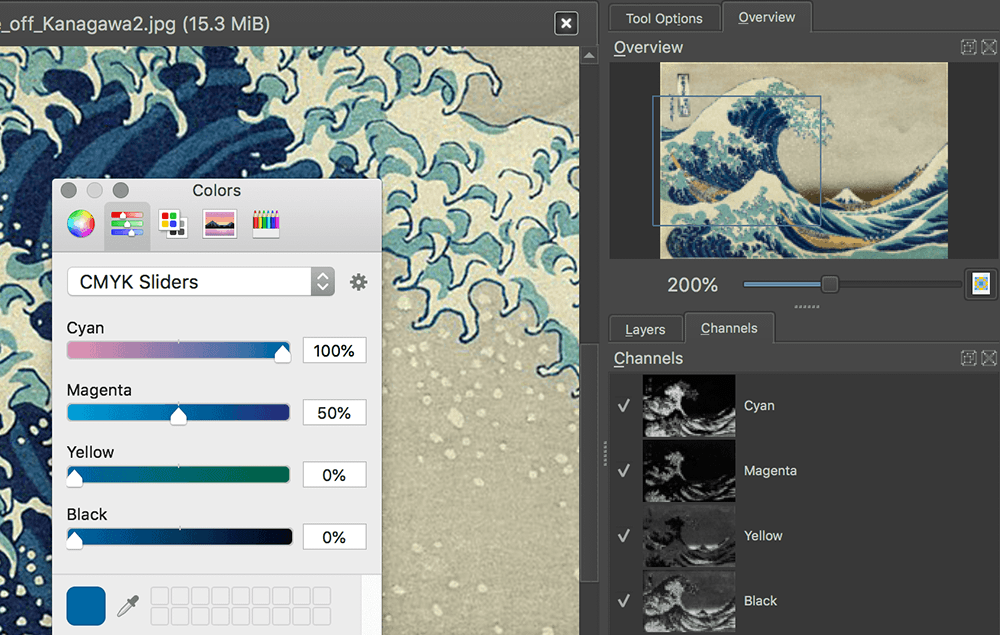
The Great Wave off Kanagawa.
Observe Krita’s Channels panel to the lower-right; whiter areas indicate higher values for the respective channel. For instance, the Cyan channel’s bright regions correspond to the blue areas in the wave. The Magenta channel appears like a duller copy of the Cyan channel; the predominant blue is mostly a mix of around 100% cyan and 50% magenta. By manipulating colour channels, you can control the overall hue, saturation, and lightness. If you are familiar with software like GIMP or Photoshop, or perhaps more basic image editing software, you’ve likely performed such operations before.
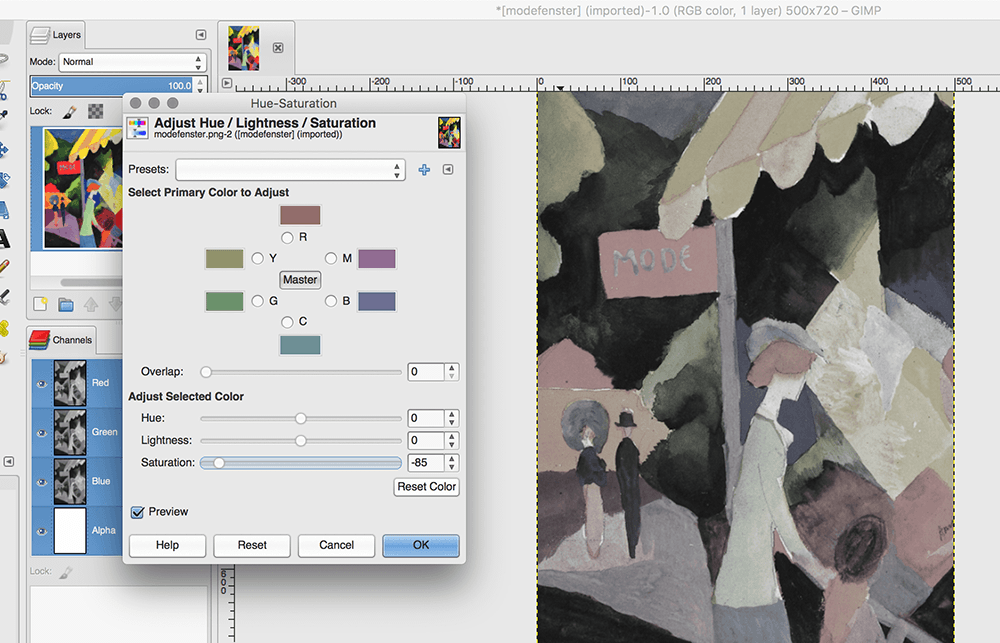
-85. GIMP's Channels panel (to the lower right) separates the image into its Red, Green, Blue, and Alpha channels.Processing has various functions for manipulating colour channels. Experimenting with these reveals the inner workings of applications like Photoshop.
RGB Channels
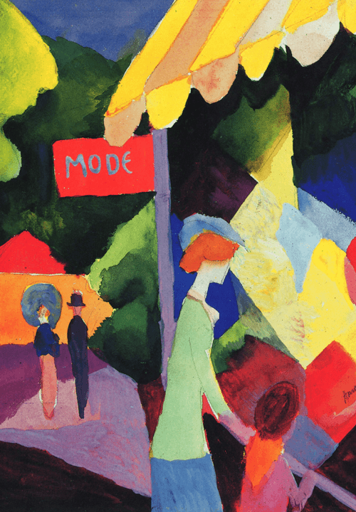
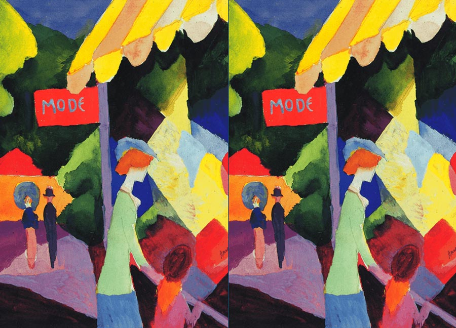
Create a new sketch and save it as “colour_channels”. Download this copy of August Macke’s Modefenster and place it your sketch’s “data” sub-directory:
Add the following setup code:
size(1000,720)
background('#004477')
noStroke()
modefenster = loadImage('modefenster.png')
image(modefenster, 0,0)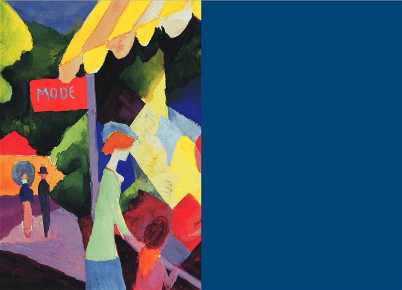
We’ll be sampling parts of the painting and placing the processed output in the empty blue area to the right. The first function you need to know is the get(). This is used to read the colours of pixels that lie within the display window. First, grab a section of pixels by adding a get() to the bottom of your code:
grab = get(0,0, 200,200)The arguments are the same as those of the rect() function; the variable grab is assigned a copy of all the pixels within a rectangular area beginning at the top left (0,0 ...) and extending 200 pixels across and 200 pixels down (... 200,200). Add an image() function to draw the pixels into the empty area on the right:
grab = get(0,0, 200,200)
image(grab, 600,100)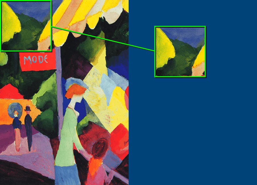
Alternatively, you can make use of the copy() function which additionally accepts arguments for the destination coordinates and scale.
#    src. coords --> dest. coords
copy(0,0,200,200,    600,600,100,100)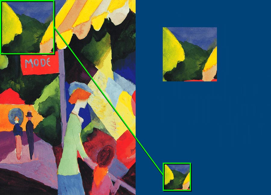
To retrieve a single pixel’s colour, use a get() function without width and height arguments. If any pixel sampled lies outside of the image window, the get() returns black.
singlepixel = get(190,200)
fill(singlepixel)
rect(700,300, 200,200)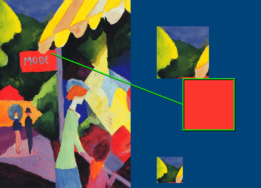
Intriguingly, if you print the singlepixel variable a (negative) integer appears; this is how Processing stores colours in memory. You do not need to understand how this works because there are functions for converting these integer-based data types to standard hexadecimal and RGB.
print(singlepixel) # -248525We can now build a duplicate image on the right by sampling each pixel and placing its clone 500 pixels (half the width of the display window) to the right. Sure, it would be easier to grab the whole area of the painting, but the pixel-by-pixel approach is necessary for the upcoming steps. Add this loop to the end of your code:
halfwidth = width/2
x = 0
y = 0

for i in range(halfwidth*height):

    if i%halfwidth==0 and i!=0:
        y += 1
        x = 0
    x += 1

    pixel = get(x,y)
    set(x+halfwidth, y, pixel)
You should be quite comfortable with loops now. In this instance, the range is half the display window’s width by the full height. In a pixel-by-pixel, row-by-row manner, the loop gets each pixel and sets its clone accordingly. The set() function accepts three arguments: an x-coordinate, then y-coordinate, then colour. Run the sketch. Your earlier experiments are drawn over with new pixels.
With each iteration, we’ll now separate the pixel values into the independent R, G, and B channels. Comment out the existing set() line and add a red(), green() and blue() function to extract the three channel values.
    ...

    pixel = get(x,y)
    #set(x+halfwidth, y, pixel)

    r = red(pixel)
    g = green(pixel)
    b = blue(pixel)
With each pixel sampled, variables r, g, and b are each assigned a value between 0 and 255. Excellent! That’s a familiar range, right? Remember, 255 equals FF equals 11111111.
The color() function converts RGB values into the integer types that get() and set() work with (the way Processing stores colours in memory). Add the following lines to the end of your loop:
    rgb = color(r, g, b)
    set( x+halfwidth, y, rgb )
Run the sketch. The result is the same as before. We have split the colour into its R/G/B constituents then merged them back together using the color() function.
Now, let’s visualise the channels beginning with red. Recall that the Channels panels in both Krita and GIMP (and Photoshop, for that matter) display greyscale thumbnails. Greys are an equal mix of red, green, and blue – therefore, to represent a red channel in greyscale, use the red value for all three color arguments.
    #rgb = color(r, g, b)
    set( x+halfwidth, y, color(r,r,r) )
If the current iteration’s pixel is bright red, the color(r, r, r) line is equivalent to color(255, 255, 255). This means that the most vivid reds will appear as white, that no red is black, and that everything else is some shade of grey. Run the code.
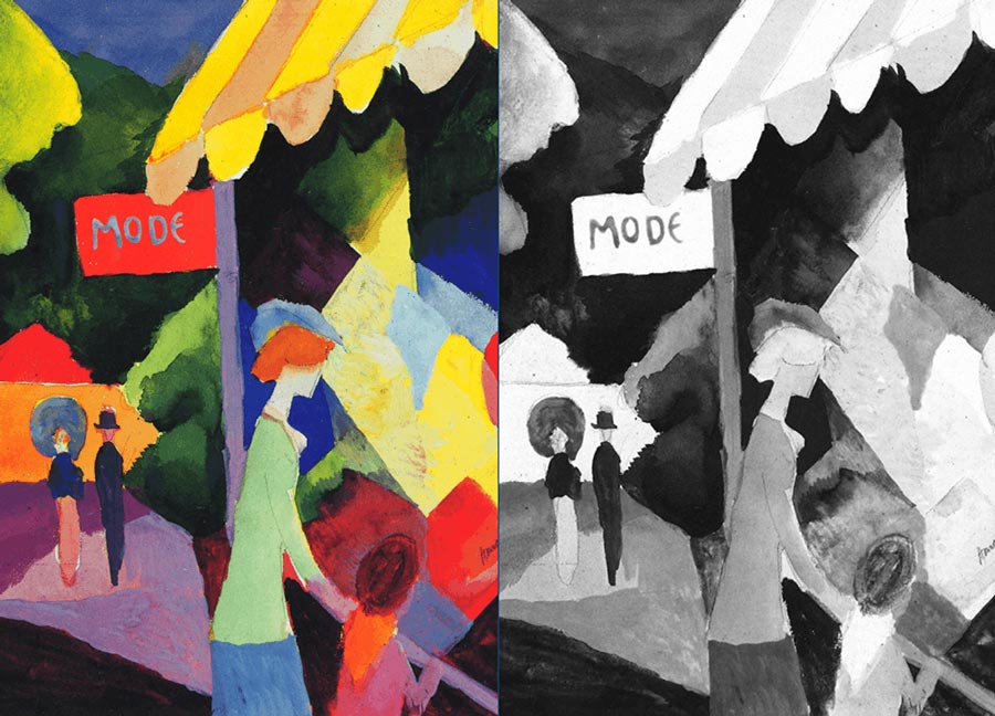
Note how the red “MODE” sign registers as white; this indicates red values of near 100%. The yellow stripes in the awning over the window are also white; this is because yellow is mixed using 100% red and 100% green. Comment out the red set() line and try a green channel instead.
    #set( x+halfwidth, y, color(r,r,r) )
    set( x+halfwidth, y, color(g,g,g) )
The green channel confirms the prominence of green in the awning. The sign, however, has very little green – or blue, for that matter. You can try a set() line for blue if you wish to confirm this. Any area in the original image that’s grey, white, or black, will possess equal quantities of red, green, and blue.
To convert the image to greyscale, rather than greyscale representations of each channel, average out the three values.
...
channelavg = (r + g + b) / 3
greyscale = color(channelavg, channelavg, channelavg)
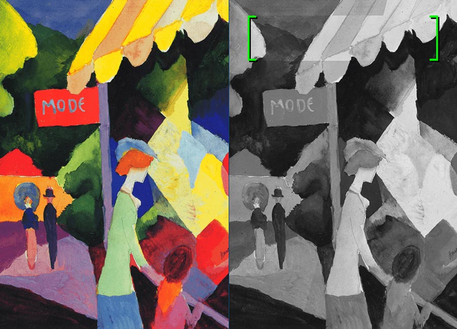
set( x+halfwidth, y, greyscale )Include the following coefficients to accommodate the greater number of green receptors in the human eye. The yellows will, otherwise, not appear bright enough.
channelavg = (r*0.89 + g*1.77 + b*0.33) / 3In the image below, the area within the green brackets exhibits the calibrated values. Note how the awning’s bright yellow and darker orange strip appear as the same shade of grey with the straightforward averaged values.
To invert the colours (like a film negative), subtract each r/g/b value from its maximum channel value of 255.
...
invcolour = color(255-r, 255-g, 255-b)
set( x+halfwidth, y, invcolour )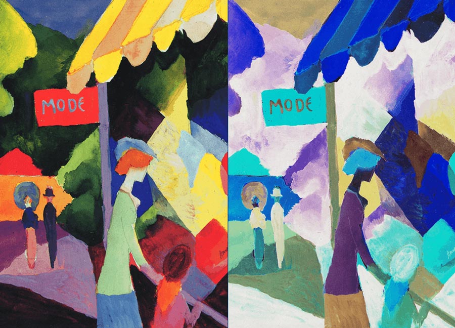
See if you can work out how to create an inverted greyscale version.
HSB Channels
Lesson 1 introduced Processing’s various colour modes. The colour mixing scheme can be switched from RGB to HSB (Hue, Saturation, Brightness) using the colorMode() function. You can think of HSB as an alternative set of channels that may be more appropriate for what you need to accomplish. Switch the colorMode to HSB and add a new loop to the end of your existing “colour_channels” code. If you wish to, you can comment out the previous loop – or instead, not bother and just allow the new loop to draw over what’s there already.
colorMode(HSB, 360, 100, 100)
x = 0
y = 0

for i in range(halfwidth*height):

    if i%halfwidth==0 and i!=0:
        y += 1
        x = 0
    x += 1
Working in HSB makes it far easier to shift hues, adjust saturation, and alter brightness. The colorMode() arguments have now set Processing to operate like the GIMP colour mixer depicted below.
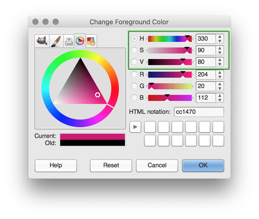
Use the hue(), saturation(), and brightness() functions to separate the pixel values into three HSB channels.
    ...
    pixel = get(x,y)
    h = hue(pixel)
    s = saturation(pixel)
    b = brightness(pixel)
To create an exact copy of the painting, use a set() line with the h/s/b variables as arguments:
set( x+halfwidth,y, color(h, s, b) )Adjusting the hue involves taking a pixel’s hue value and rotating the GIMP mixer triangle to produce a new rotation value between 0 and 360 degrees. This is akin to shifting a hue slider in GIMP or Photoshop.
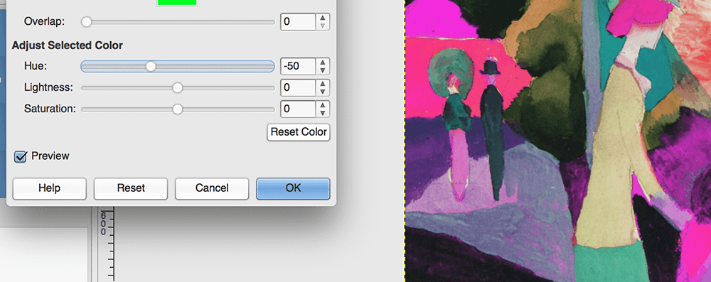
But simply adding degrees of rotation to the h variable is problematic. For example, what if the h is 40 and we subtracted 50. The result is 40 - 50 = -10 degrees, which lands outside of the permitted range. Instead, rotating past 0 or 360 should reset the degrees to zero, then subtract/add the remaining difference. This way 40 - 50 = 350 degrees. This is an example of clock arithmetic. The ‘wrap-around’ concept is nothing new to you. If it’s currently three AM, and somebody asks what time was it four hours ago, you’dn’t say “minus one AM”? Clock arithmetic is an application of modular arithmetic – the favourite pastime of our good friend the modulo operator! Add a new set() line that subtracts 50 from the hue and performs a %360 on the result.
    #set( x+halfwidth,y, color(h, s, b) )
    set( x+halfwidth,y, color((h-50)%360, s, b) )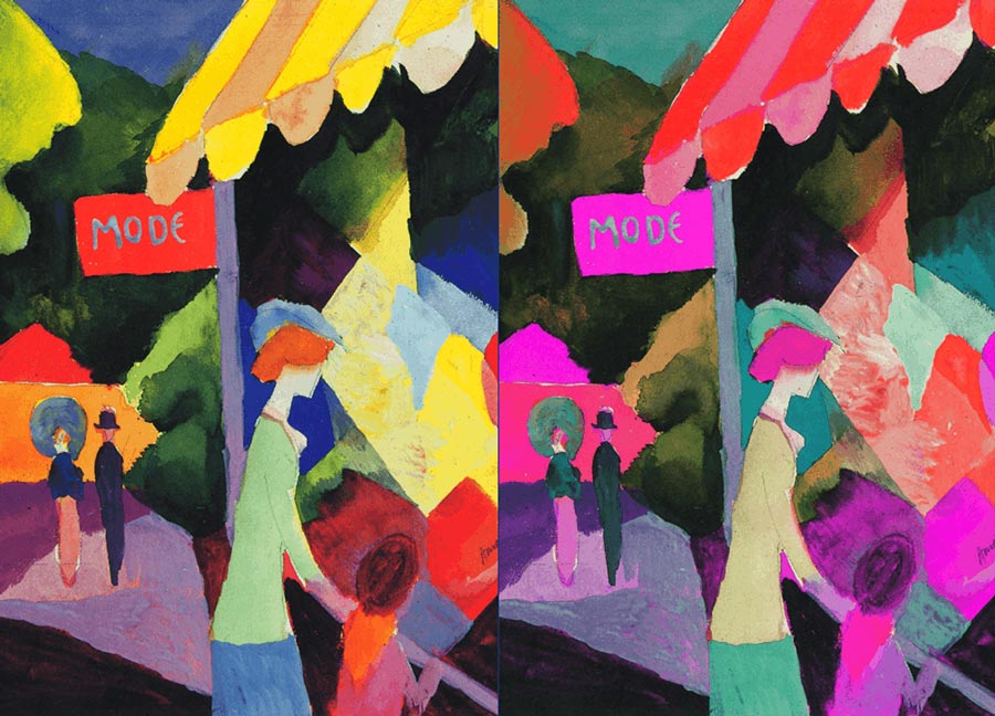
To invert the colour, but keep the same brightness, pick the colour on the opposite side of the colour wheel by adding 180°.
set( x+halfwidth,y, color((h+180)%360, s, b) )For the most vivid colours possible, set the saturation value to maximum (100%) for every pixel.
set( x+halfwidth,y, color(h, 100, b) )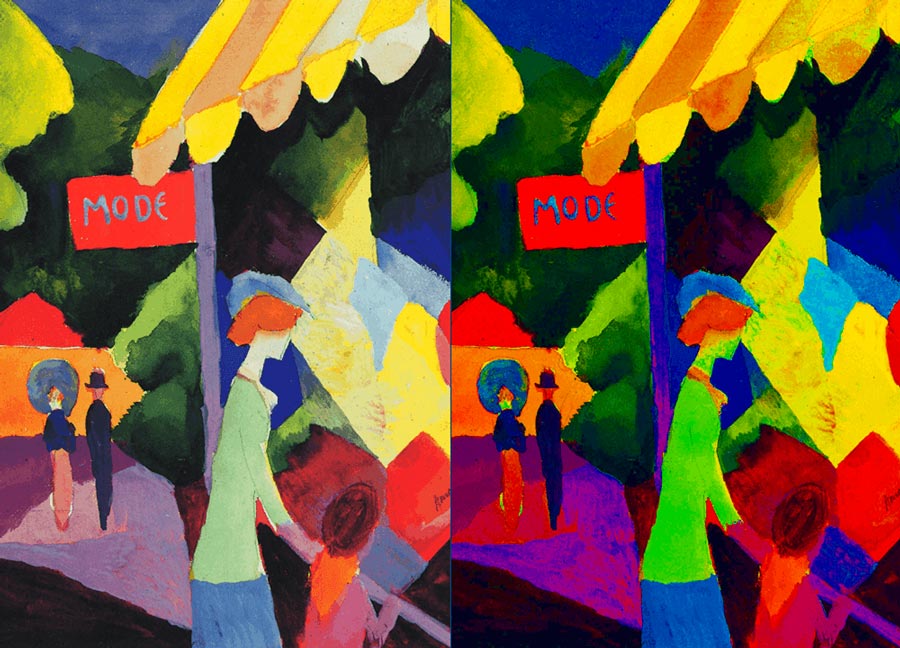
You are now familiar with colour channel management. You can apply this theory to all sorts of colour adjustment. These principles also lay the foundation for the next sections where we look at filter effects. There are a few other functions for the colour data type that we did not cover. These omissions include:
alpha(), for extracting alpha (transparency) values;blendColor(), for blending two colours using a selection of modes;lerpColor(), for calculating the colour(s) that lie between two other colours;loadPixels(),pixels(), andupdatePixels(), which work together to load and manipulate pixels in the display window. This is a faster, albeit more complicated, alternative to usingget()andset().
6.3: Halftones »
Complete list of Processing.py lessons