« 6.2: Colour Channels |
6.4: Image Kernels »
Halftones
Suppose that you’ve an image of continuous tones, i.e. an infinite-like range of blended greys. For this example, we’ll use a photograph of Elisabet Ney’s Lady Macbeth sculpture (below). The image is to appear in a newspaper printed in black & white, so you convert the image to greyscale and email it off to the publishers.
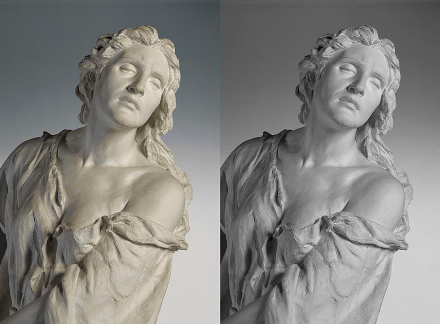
Lady Macbethin colour and greyscale.
Ingrid Fisch [CC BY-SA 3.0]
Of course, in the 1870s it wasn’t this simple. There was no email and, more critically, publishers were still figuring how to print photographs. In spite of this limitation, printers managed to reproduce illustrations. Illustrations were etched into wood then cast into metal plates; which could then be coated in ink and used to transfer the images to paper. The challenge with photographs was continuous tones – or more specifically, how to render solid black ink in a multitude of grey shades. The solution was halftone; tiny dots of varying size that create the illusion of grey when viewed from a sufficient distance. The exact details of the process are not important; suffice to say it’s all handled digitally today.
The images below contrast four different halftone techniques. The simplest approach is no halftone (top-left). Here, a brightness threshold is used to determine which shades of grey are rendered black or white. The stochastic halftone (top-right) uses dots of equal size, adjusting their spacing to emulate darker/lighter tones. Such dithering techniques can, therefore, be described as frequency modulated.
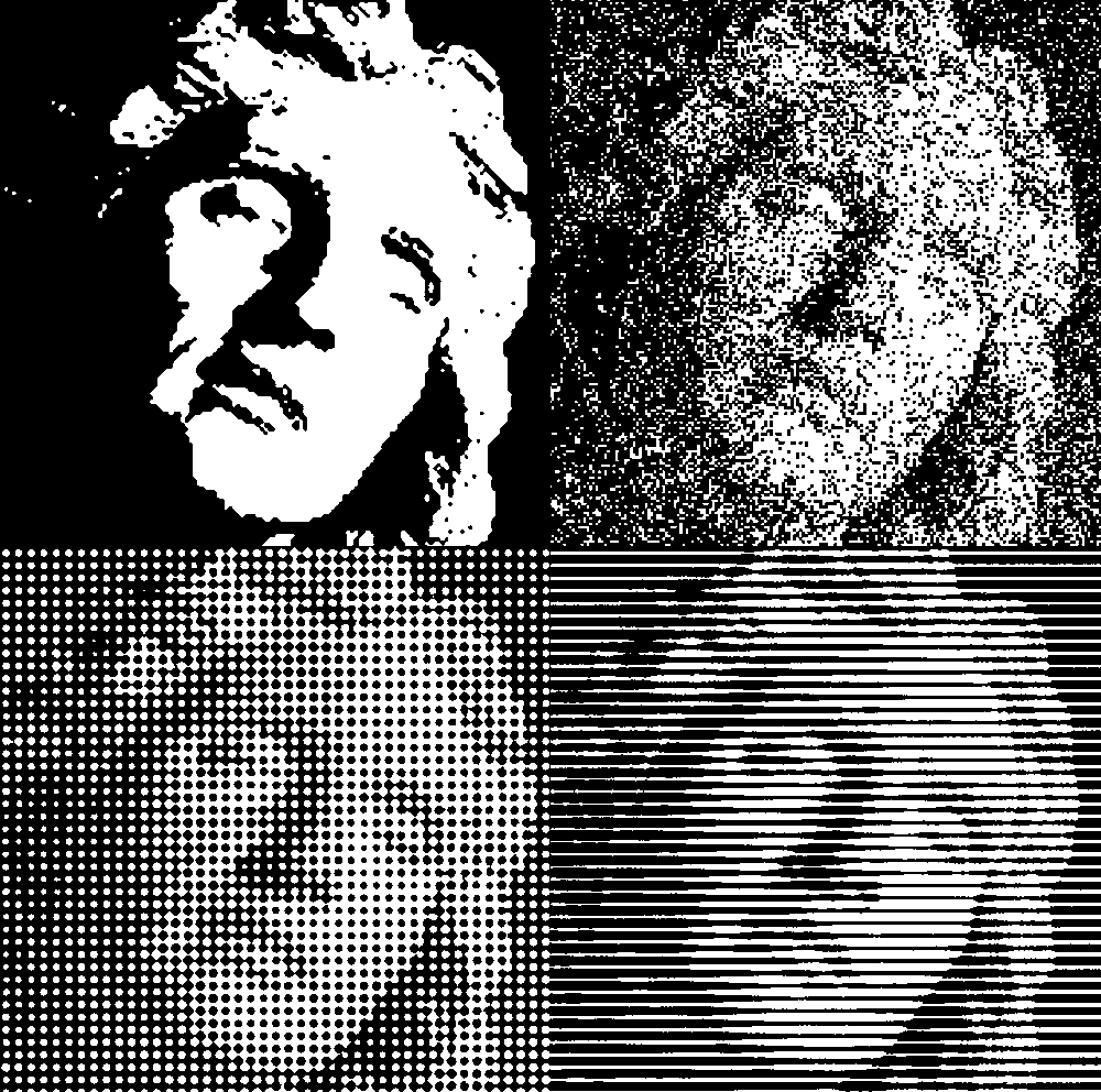
Amplitude modulated halftones (bottom-left and bottom-right) rely on varying sized dots in a grid-like arrangement, or evenly-spaced lines of variable weight. These patterns, however, can be formed using various other shapes (squares, ellipses, etc.).
Halftone techniques remain an essential part of printing today. Halftone separations for each CMYK channel create the optical effect of full-colour imagery when overlayed as semi-opaque inks.

Pbroks13d (SVG version) and Slippens (PNG original) [Public domain], via Wikimedia Commons
Round dots are the most commonly used shapes. If you magnify a print you should be able to spot them.
Halftone Dots
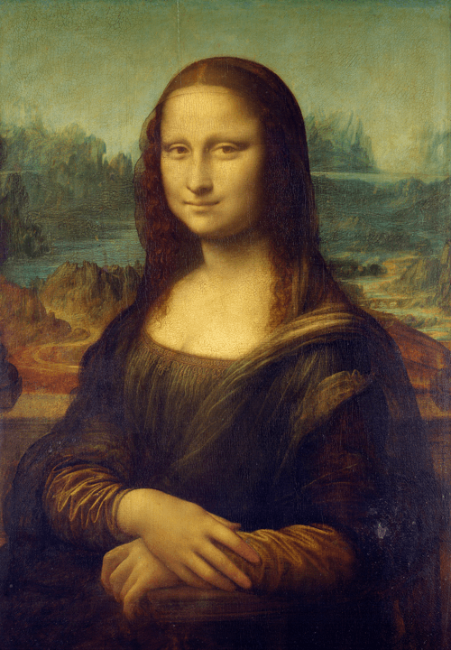
Create a new sketch and save it as “halftones”. Download this copy of Leonardo da Vinci’s Mona Lisa and place it your sketch’s “data” sub-directory:
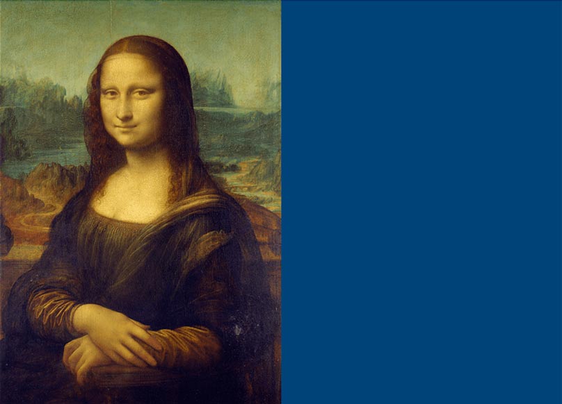
Add the following setup code:
size(1000,720)
background('#004477')
noFill()
monalisa = loadImage('mona-lisa.png')
image(monalisa, 0,0)
As with the previous sketch, we’ll be rendering a processed version in the empty blue space on the right.
Our first halftone will consist of amplitude-modulated circles. We’ll begin by adding the global variables and main loop. The image will be divided into ‘cells’. In effect, these cells control the ‘resolution’ of the halftone.
halfwidth = width/2
coltotal = 50.0                  # number of cells per row
cellsize = halfwidth/coltotal    # width/height of each cell
rowtotal = ceil(height/cellsize) # cells per column
col = 0
row = 0

for i in range( int(coltotal*rowtotal) ):

    x = int(col*cellsize)
    y = int(row*cellsize)
    col += 1

    if col >= coltotal:
        col = 0
        row += 1

    rect(x,y, cellsize,cellsize)
Most of this code should look familiar, although the ceil() function may be new to you. The ceiling function performs a round-up operation on floating point values. For example, ceil(9.1) would return 10. It’s necessary to employ it here to prevent any half rows from stopping short of the bottom of the display window. A rect() line is included to visualise the cells. Run the code.
For the halftone effect, we want to sample the pixel a the centre of each cell. To accomplish this, add half the width/height to the x/y coordinate. Also, comment out the rect() line.
    #rect(x,y, cellsize,cellsize)
    x = int(x+cellsize/2)
    y = int(y+cellsize/2)
    pixel = get(x,y)
Next, using the brightness value of each pixel sampled, we calculate an amplitude (amp) for each halftone dot. The amount, however, must be reduced by a factor of 200 so that the dots are not too large.
    ...
    pixel = get(x,y)
    b = brightness(pixel)
    amp = 10*b/200.0
Finally, add the relevant stroke and fill properties, then the ellipse/circle function.
    noStroke()
    fill('#FFFFFF')
    ellipse(x+halfwidth,y, amp,amp)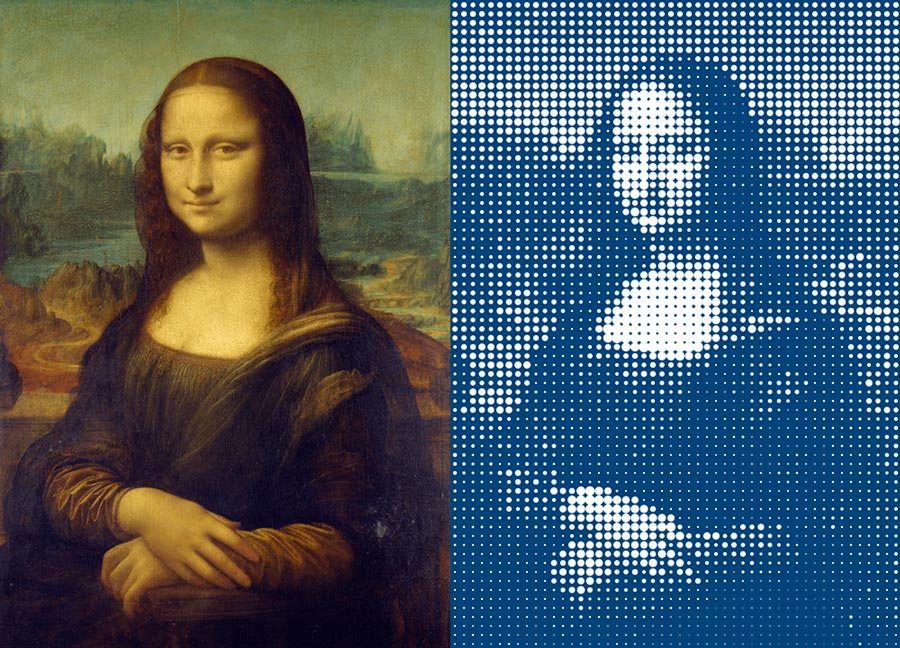
You are not limited to circles or white fills. In the next two tasks, you’ll be challenged to replicate two new halftone effects.
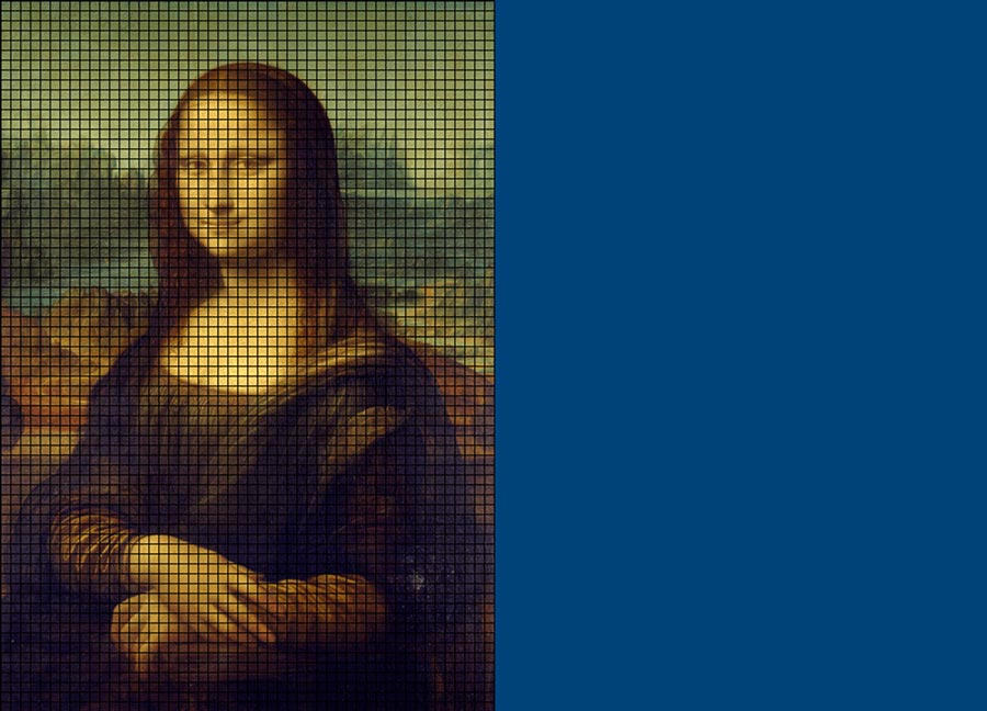
Pixel Art Task
Using the “haltones” sketch you’ve been working on, recreate the pixelated effect below.
You should be able to comment out the circular-halftone-specific lines and make use of the existing loop.
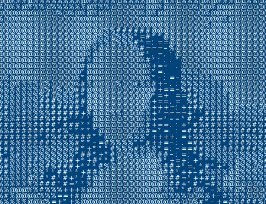
ASCII Art Task
For ASCII art, you’ll need to decide on a set of characters to serve as your colour ramp. For ten shades, you can use the following sequence (which begins with a space character). The glyphs range from lightest on the left to darkest at the right.
` .:-=+*#%@`
With so few shades, expect substantial posterisation – the “conversion of a continuous gradation of tone to several regions of fewer tones, with abrupt changes from one tone to another” (Wikipedia). The final result should look something like this:
There are many halftone effects to explore. By riffing off the techniques covered here, you can come up with all sorts of interesting results. For example, see what happens when you combine the circular, pixel, and ASCII effects.
6.4: Image Kernels »
Complete list of Processing.py lessons