« 6.3: Halftones |
6.5: Filters and Blends »
Image Kernels
If you’ve ever sharpened or blurred a digital image, it’s likely that the software you were using relied on an image kernel to process the effect. Moreover, the fields of computer vision and machine learning utilise image kernels for feature- detection and extraction.
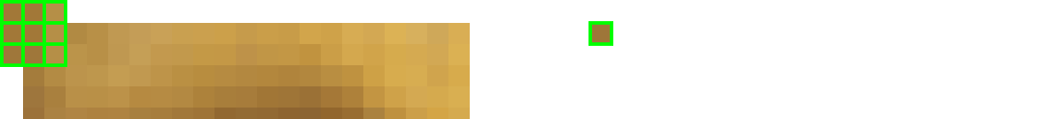
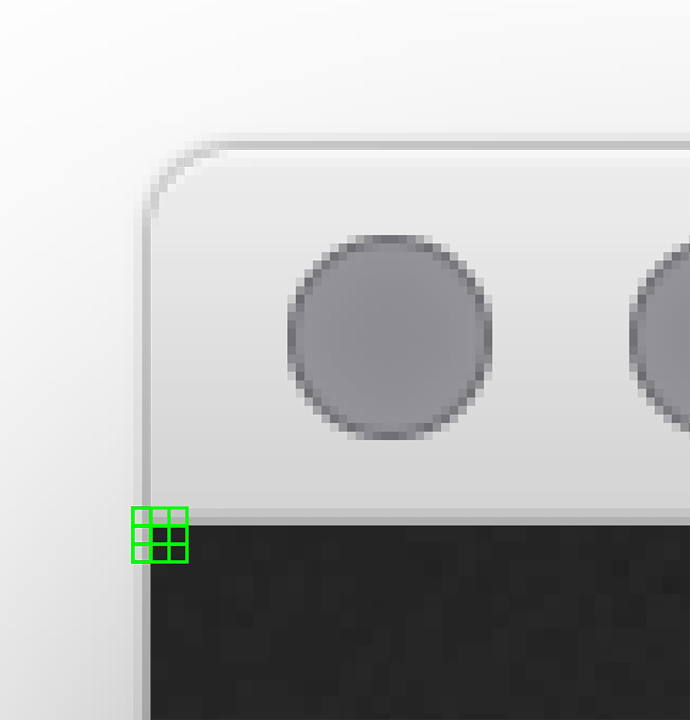
An image kernel, put simply, is a small matrix that passes over the pixels of your image manipulating the values as it moves along. To illustrate, here’s a three-by-three blur kernel in action. The kernel (left) begins with its centre placed over the first (top-left) pixel of the source image. A new (first) pixel value is calculated using the centre and eight neighbouring cells sampled in the kernel.
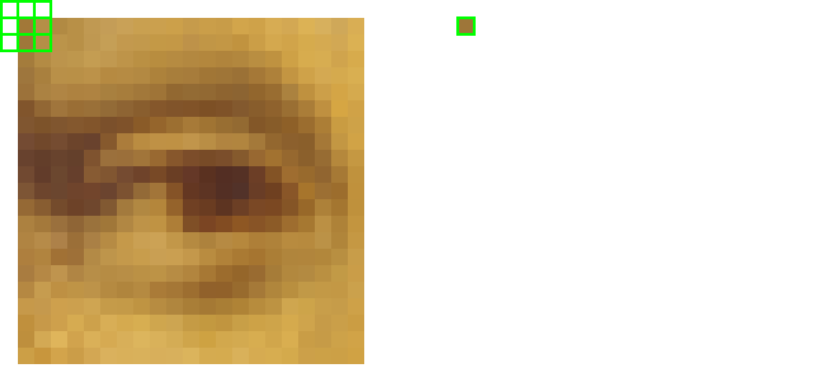
For any edge pixels, though, the kernel ‘hangs’ over the boundary and samples empty cells. One common solution is to extend the borders pixels outward.
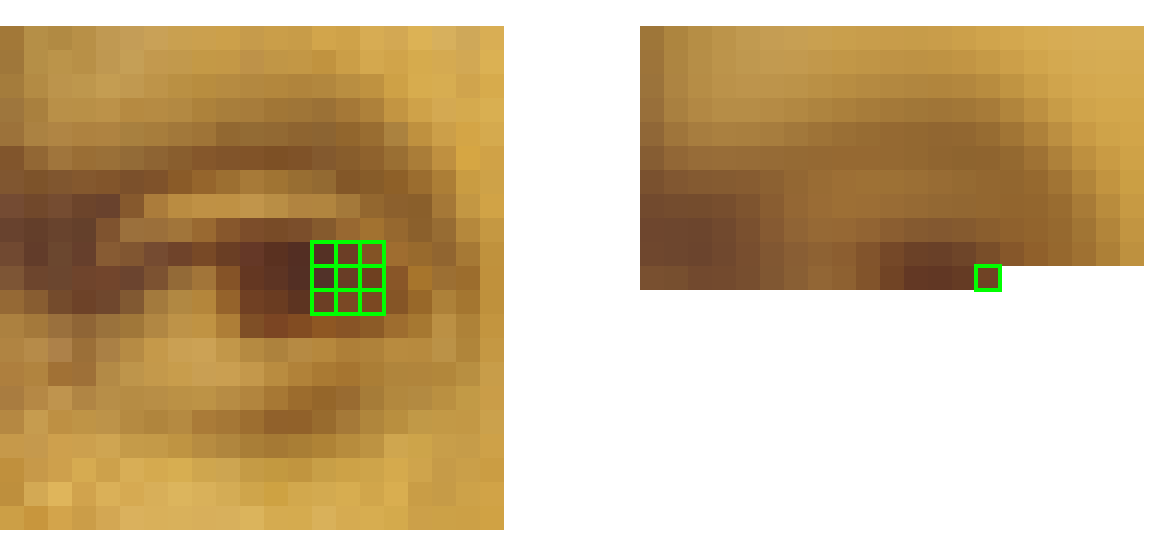
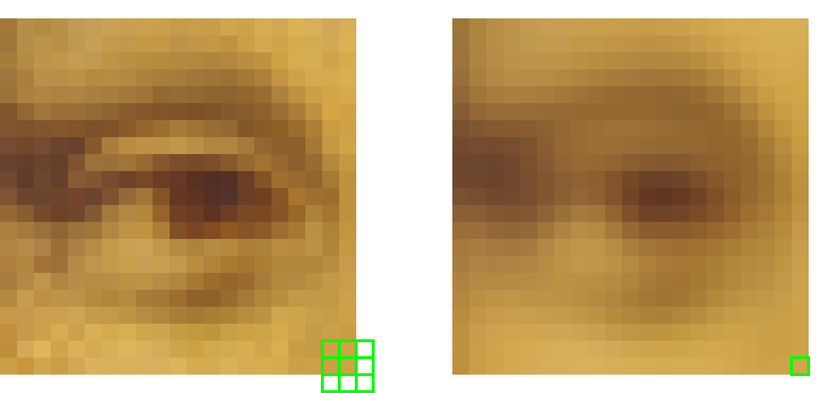
This process advances pixel-by-pixel. In this instance, the kernel motion is left-to-right, row-by-row – although, as long as every pixel is processed, the sequence does not matter.
The magic part is how the kernel combines the nine values into one – a form of mathematical convolution, where each pixel is weighted and then added to its local neighbours. In the illustration below, the source pixels are labelled a–i and the matrix cells, 1–9.
The convolution operation multiplies each cell by its corresponding partner. So, a × 1, then b × 2, and so on through to i × 9. The results of all these multiplications are then added together, producing a blurred colour value.
If you are a math/ML/CV/other nerd – you may point out that that kernel has not been flipped, so this is, in fact, a cross-correlation and not a convolution. You are correct. However, we’ll be using symmetrical kernels, so correlation and convolution coincide.
The numbers 1–9 are simply variables. With the theory out of the way, it’s time to program your own image kernels so that you can experiment with different combinations of weightings.
Roll Your Own Image Kernel
Create a new sketch and save it as “image_kernels”.
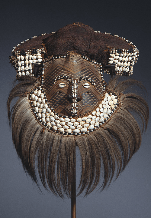
Download this image of a Kuba people’s Mwaash aMbooy mask and place it your sketch’s “data” sub-directory:
Begin with the following code:
size(1000,720)
background('#004477')
noStroke()
mwaashambooy = loadImage('mwaash-ambooy-grey.png')
image(mwaashambooy, 0,0)
The image has been greyscaled prior to loading. A single colour channel will be easier to manage at first.
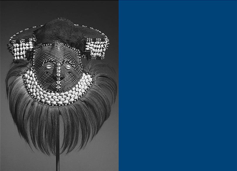
Brooklyn Museum [CC BY 3.0 / converted to greyscale]
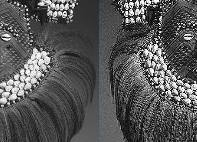
As with the previous tasks, the processed version will appear in the blue area to the right. To begin, add a loop to your sketch.
halfwidth = width/2
x = 0
y = 0

for i in range(halfwidth*height):

    if i%halfwidth==0 and i!=0:
        y += 1
        x = 0
    x += 1
Because we are sampling greyscale pixels, it does not matter if you extract the red, green, or blue channel – remember that these are equal for any shade of grey. Add the following line to the loop:
sample = red( get(x,y) )Next, create a new grey color, assign it to a variable named kernel, and use set to draw a corresponding pixel in the right half of the window:
    kernel = color(sample,sample,sample)

    set(x+halfwidth, y, kernel)
We could use a get(x,y) as the third argument of the set() function and thereby forgo the previous two lines. The visual result is an exact duplicate of the source, anyhow. The purpose of these seemingly unnecessary steps is to verify that everything works for now; we’ll adapt this code as we go.
With each iteration, we must sample nine pixels for the kernel. The loop begins at the top-left pixel, meaning that, on the first iteration the kernel samples five ‘empty’ pixels that lie beyond the edges. To keep things simple, we’ll not use the ‘extend’ trick; rather, Processing will record these as black. This will result in slightly darkened border pixels, but nothing too noticeable.
Replace the sample variable with a list. This new list structure grabs the nine pixels at once.
    #sample = red( get(x,y) )
    sample = [
      red(get(x-1,y-1)), red(get(x,y-1)), red(get(x+1,y-1)),
      red(get(x-1,y))  , red(get(x,y))  , red(get(x+1,y)),
      red(get(x-1,y+1)), red(get(x,y+1)), red(get(x+1,y+1))
    ]
Next, replace the kernel variable with a list that multiplies the sample values by some kernel weightings. To start, we’ll perform an identity operation – which is math-speak for “returns the same values it was provided”.
    #kernel = color(sample,sample,sample)
    kernel = [
      0*sample[0], 0*sample[1], 0*sample[2],
      0*sample[3], 1*sample[4], 0*sample[5],
      0*sample[6], 0*sample[7], 0*sample[8]
    ]
To illustrate this operation using the matrix diagram from earlier – we have black left/top edge pixels and a matrix of zeroes with a 1 in the centre.
Recall though, that after multiplying, we add-together the products. The Python sum() function makes things easy for you, adding up all the numbers in a list. Replace the existing set line as below.
#set(x+halfwidth, y, kernel)
r = sum(kernel)
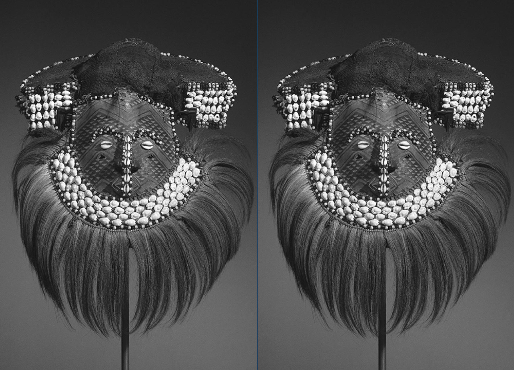
set( x+halfwidth, y, color(r, r, r) )Run the sketch. The results appear the same as before (an exact duplicate). You are now ready to begin experimenting with different kernel weightings.
Box Blur
The box blur is a simple kernel that averages adjacent pixel values. The result is a ‘softer’ image with lower contrast.
    kernel = [
      0.11*sample[0], 0.11*sample[1], 0.11*sample[2],
      0.11*sample[3], 0.11*sample[4], 0.11*sample[5],
      0.11*sample[6], 0.11*sample[7], 0.11*sample[8]
    ]
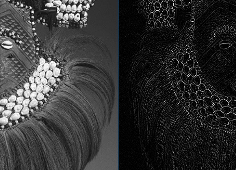
Edge Detection
As the name implies, edge detection methods aim to identify edge points/boundaries within an image. The lighter the resultant pixel appears, the more pronounced the change is in image brightness.
    kernel = [
      0*sample[0], 1*sample[1], 0*sample[2],
      1*sample[3],-4*sample[4], 1*sample[5],
      0*sample[6], 1*sample[7], 0*sample[8]
    ]
Sharpen
Sharpening makes light pixels lighter and dark pixels darker. The result is an increased contrast and ‘crisper’ edges. The kernel is, effectively, the inverse of an edge detect.
    kernel = [
      0*sample[0],-1*sample[1], 0*sample[2],
     -1*sample[3], 5*sample[4],-1*sample[5],
      0*sample[6],-1*sample[7], 0*sample[8]
    ]
These are a few common kernel types. However, image kernels need not be limited to 3 × 3, symmetric matrices and can operate on whatever channel(s) you feed them (full-colour RGB, HSB, etc.). Like many things matrix-related, this stuff can get very involved. We’ll not venture any deeper, although the final section of lesson 6 covers Processing’s filter functions, many of which rely on convolution matrices.
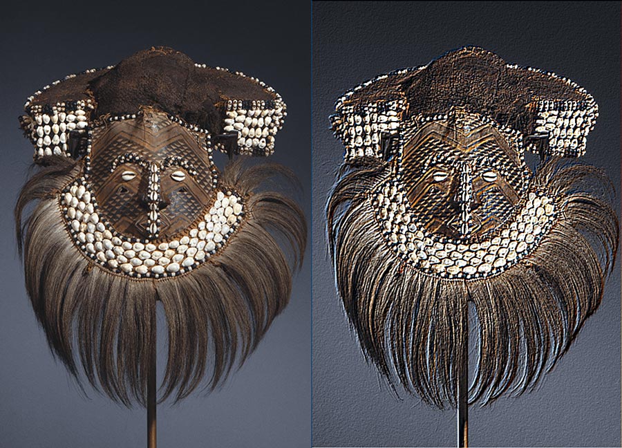
Colour Emboss Task
In this task, the challenge is to apply an emboss to a colour image. You may use your existing sketch or create a new one. Download the colour version of the Mwaash aMbooy mask and place it your sketch’s “data” sub-directory:
Do not forget to load the colour image:
...
mwaashambooy = loadImage('mwaash-ambooy-colour.png')
image(mwaashambooy, 0,0)
...
The emboss kernel creates the illusion of depth by emphasising contrast in a given direction.
The final result looks like this:
If you’ve no idea where to start, consider a separate kernel for each R/G/B channel.
6.5: Filters and Blends »
Complete list of Processing.py lessons