« 6.4: Image Kernels |
6.6: Tint and Transparency »
Filters and Blends
If you are a user of raster graphics software, such as GIMP or Photoshop, you’ve almost certainly encountered filters and blend modes. On a technical level, blend modes – and most filters – operate on colour channels. Processing’s filter and blend functions span a selection of common image processing algorithms. Technically speaking, one can program these effects using the techniques covered thus far. We look at replicating a few of the simpler blend modes.
Filters
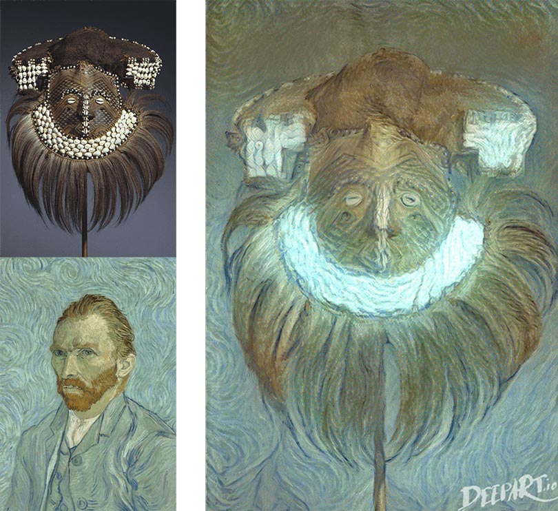
Filters range from utilitarian and understated to hideously gaudy. To be fair, most have their place, but perhaps some users lack an understanding of how much of – and to which parts of an image – a given filter should be applied. Some impressive developments are being made in this area thanks in part to advances in artificial intelligence. For instance, here’s a Vincent van Gogh imitation of the Mwaash aMbooy mask created using DeepArt.io’s neural algorithm.
Rather than list all of GIMP’s filters, here are the top-level categories into which they are arranged: blur, enhance, distort, light and shadow, noise, edge detect, generic, combine, artistic, decor, map, render, web, and animation. On average, a category contains around ten items, so that’s a lot of filters! Processing has eight filters in total.
The Processing filter() function requires a predefined filter name as an argument. Depending on the effect, there may be a second argument. If you want to experiment, download this photo of Florentijn Hofman’s Rubber Duck. Alternatively, you may prefer just to read over this section. The tutorial provides an image comparing all of the effects further along.
480px-Rubber_Duck_in_Sydney,_January_5,_2013.jpg
If you’ve decided to write some code, place the image in the sketch’s “data” sub-directory and add the following code:
size(480,480)
background('#004477')
rubberduck = loadImage(
  '480px-Rubber_Duck_in_Sydney,_January_5,_2013.jpg'
)
image(rubberduck, 0,0)
textSize(28)
text('Rubber Duck', 20,150)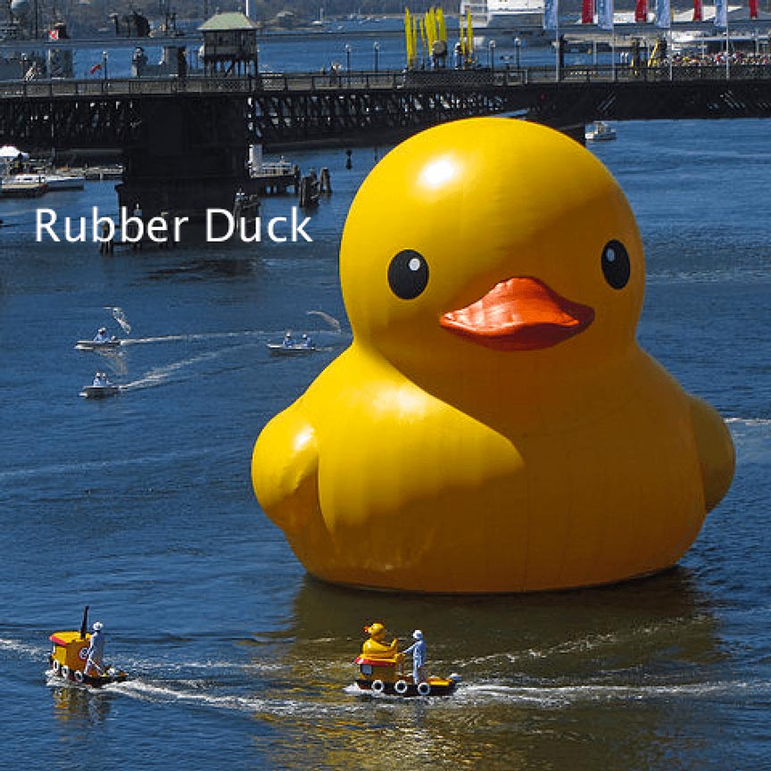
Rubber Duckby Florentijn Hofman, in Darling Harbour as part of the 2013 Sydney Festival.
Newtown grafitti [CC BY 2.0 / added title], via Wikimedia Commons
To blur the image, add the following line to the end of your code:
filter(BLUR)For more blurring, BLUR accepts an additional level parameter. For example:
filter(BLUR, 3)The array of images below compares each of Processing’s filter arguments. The caption beneath lists the corresponding function calls.
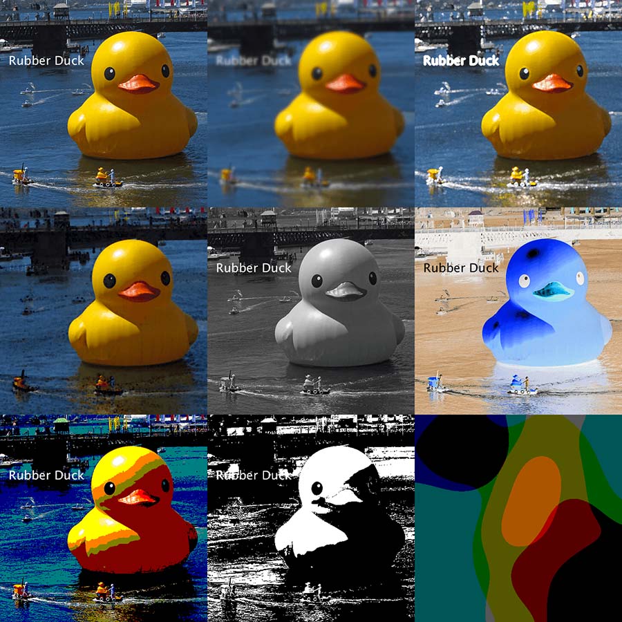
filter(BLUR,3)filter(DILATE) × 2filter(ERODE) × 2filter(GRAY)filter(INVERT)filter(POSTERIZE,3)filter(THRESHOLD)You already know how to program a number of these filters manually. If you are wondering how DILATE works, it’s a kernel that replaces the matrix centre pixel with its brightest neighbour; the ERODE, on the other hand, picks the darkest. Note that the effect manipulates everything drawn before the filter() line. Any subsequent code is unaffected. For example:
...
filter(BLUR)
textSize(15)
text('Sydney, 2013', 20,180)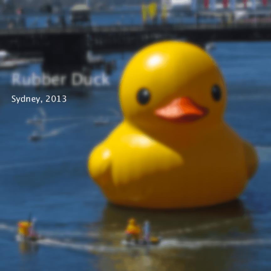
Sydney, 2013line comes after the filter function and is therefore unaffected.
If you are using animation, the filter effects become cumulative. In other words, a filter(BLUR) placed within a draw() block results in an image that’s blurred more and more with each frame.
By combining multiple built-in filters, your own programmed effects, and even some animation, you can create some mesmerising effects. Explore the GIMP/Photoshop/Krita/etc. filters for more inspiration.
Image Blend Modes
When I began using raster graphics software (Photoshop 5.5 in 1999) I was thrilled with how I could manipulate photographs using a variety of touch-up, filter, and distortion tools. Initially, blend modes were something I seemed to gloss over and never touch again. In time, though, I grew more accustomed to incorporating them in my workflow. Today, I swear by them. Before, I had always found their names confusing and never understood which blend to select for the desired effect. Most of the time I’d simply cycle through them until I struck the right look. When I eventually learnt about the underlying math, everything made sense.
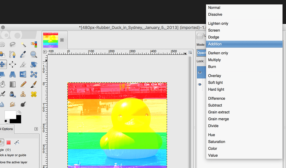
If you’ve no experience with blend modes, the screenshot below should help explain how they work. Let me begin by stating that layers are an integral component of raster graphic applications. Elements are placed on different layers so that they can be moved, scaled, and reordered to form a desired composition. By default, layers are opaque, obscuring any elements that lie further down the ‘stack’. By adjusting the blending mode, you control how the lower layers are affected. For example, a multiply blend mode has a tint-like effect.
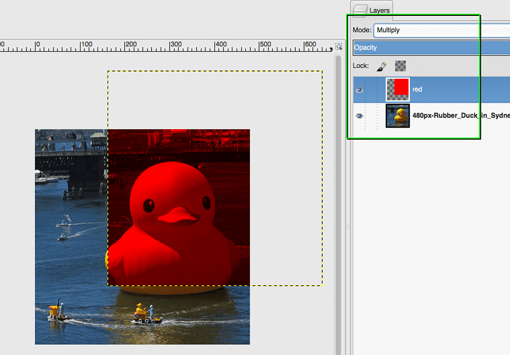
redlayer has its blend
Modeset to Multiply.
Perhaps you’ve never used blend modes. Or, maybe you’re that Photoshop whiz who intuitively selects modes but can’t begin to explain how they work? Today, we unravel the mystery.
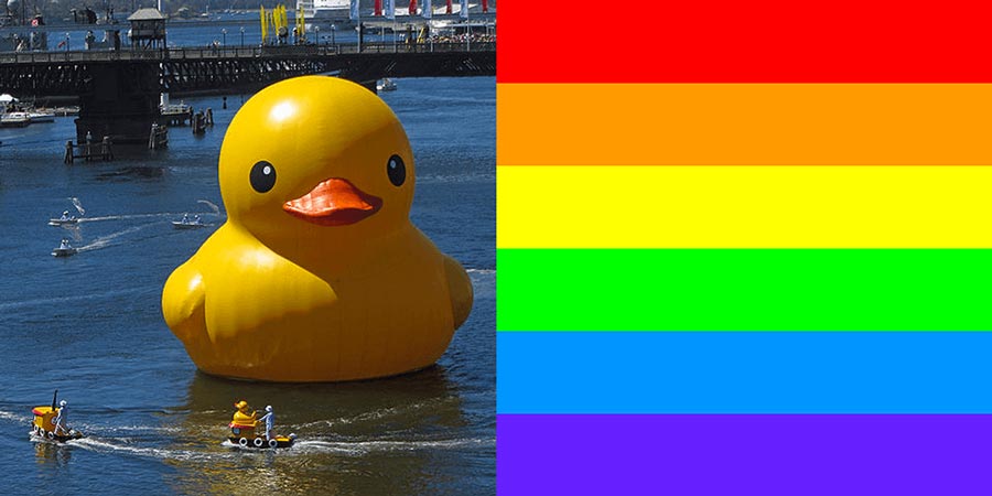
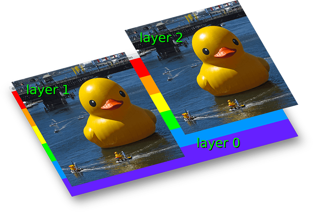
We’ll begin by programming our own blend mode, then move onto Processing’s built-in functions. Create a new sketch and save it as “blends”. In the “data” sub-directory, add a copy of the Rubber Duck image file from the last exercise. Add some code to draw a sequence of rainbow bands and place the image.
size(960,480)
background('#004477')
noStroke()
halfwidth = width/2

fill('#FF0000'); rect(0,0,width,80)
fill('#FF9900'); rect(0,80,width,80)
fill('#FFFF00'); rect(0,160,width,80)
fill('#00FF00'); rect(0,240,width,80)
fill('#0099FF'); rect(0,320,width,80)
fill('#6633FF'); rect(0,400,width,80)

rubberduck = loadImage(
  '480px-Rubber_Duck_in_Sydney,_January_5,_2013.jpg'
)
image(rubberduck, 0,0)
Run the sketch and confirm that the visual output matches the image below.
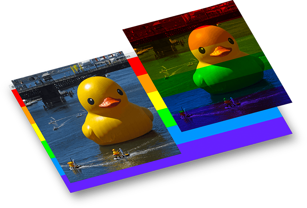
As with the previous exercises, a duplicate of the duck will be drawn to the right – in this case, over the rainbow colours. The difference this time will be the blending modes you apply in the process. Start by setting the colorMode’s RGB values so that they range from 0–1 (as opposed to the default 0–255).
colorMode(RGB, 1)In this new mixing scheme, bright red is color(1,0,0)
This will help when it comes to performing blend mode calculations.
Next, use a loop to draw an exact duplicate to the right.
x = 0
y = 0

for i in range(halfwidth*height):

    if i%halfwidth==0 and i!=0:
        y += 1
        x = 0
    x += 1

    layer1 = get(x, y)
    r = red(layer1)
    g = green(layer1)
    b = blue(layer1)
    layer2 = color(r, g, b)
    set( x+halfwidth, y, layer2 )
Splitting the layer1 value into its composite channels only to recombine them seems redundant, but structures the code for the upcoming steps. Run the code to confirm the correct visual output.
This is the simplest blend mode, normal, where the upper ‘layer’ completely conceals everything beneath it (the rainbow colours). We may not have actual layers, but can conceptually visualise the idea as such:
From here onward, we’ll make adjustments to the r/g/b variables to achieve different blends. Let’s try a multiply. Multiply gets its name from the arithmetic involved, whereby the corresponding channel values of the upper and lower layers are multiplied together. Adapt your code:
    ...
    layer1 = get(x, y)

    layer0 = get(x+halfwidth, y)
    r = red(layer0) * red(layer1)
    g = green(layer0) * green(layer1)
    b = blue(layer0) * blue(layer1)

    layer2 = color(r, g, b)
    ...
The result is a rainbow-sequence of colour tints.
I’m sure that you can guess how the add, and subtract modes work? While you can manually program your own blend modes, it’s easier to reach for Processing’s blend() and blendMode() functions. The blend() has a few more options, but blendMode() is the approach recommended by Processing’s developers. Below is a table of the various blendMode() arguments/modes and their calculations on the red channel. Of course, blue and green channels would be likewise affected.
BLEND |
the default/normal blend mode | |
ADD |
r = red(layer0) + red(layer1) |
|
DARKEST |
r = min( red(layer0), red(layer1) ) |
|
DIFFERENCE |
SUBTRACT that switches operands to always get a positive value |
|
EXCLUSION |
DIFFERENCE with a lower contrast |
|
LIGHTEST |
r = max( red(layer0), red(layer1) ) |
|
MULTIPLY |
r = red(layer0) * red(layer1) |
|
REPLACE |
BLEND with no alpha support |
|
SCREEN |
r = 1-(1-red(layer0)) * (1-red(layer1)) |
|
SUBTRACT |
r = red(layer0) - red(layer1) |
|
The following image compares each of above-listed modes – beginning with BLEND at the top-left, then proceeding left-to-right, row-by-row, ending on SUBTRACT at the bottom-right.
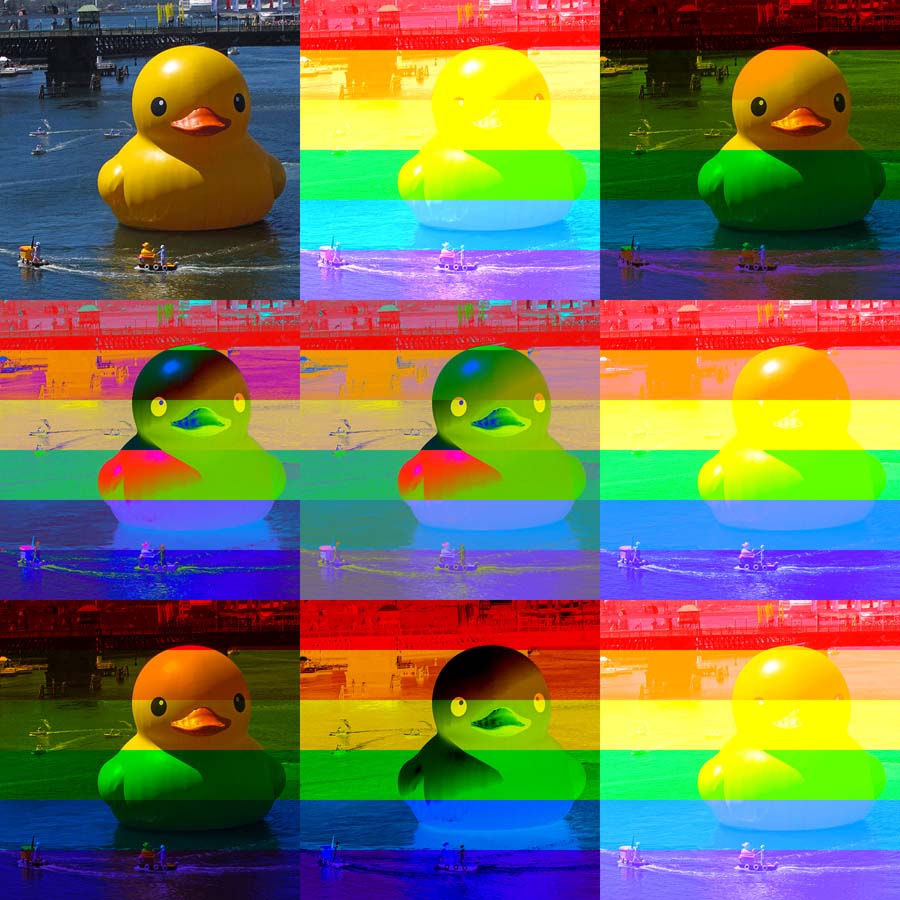
blendMode(BLEND)blendMode(ADD)blendMode(DARKEST)blendMode(DIFFERENCE)blendMode(EXCLUSION)blendMode(LIGHTEST)blendMode(MULTIPLY)blendMode(SUBTRACT)blendMode(SCREEN)You can replace the entire for loop with this blend() and image() function.
blendMode(MULTIPLY)
image(rubberduck, halfwidth,0)
'''
x = 0
...
Be aware, though, the blend mode will persist for any subsequent images or shapes that you draw. For example:
blendMode(MULTIPLY)
image(rubberduck, halfwidth,0)
fill('#FF0000')
ellipse(halfwidth,height/2, 300,300)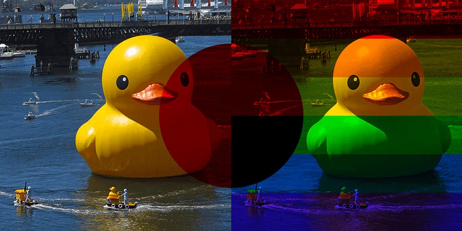
blendMode(MULTIPLY) line exhibits multiply behaviour.
To ‘reset’ to the default, use the blendMode argument, BLEND
    blendMode(MULTIPLY)
    image(rubberduck, halfwidth,0)
    fill('#FF0000')
    ellipse(halfwidth,height/2, 300,300)
    blendMode(BLEND)
    # back to normal hereafter ...
Graphic designers, VFX artists, and animators rely on blending modes for many neat tricks. For instance, multiply and subtract are handy for extracting logos from white or black backgrounds; darkest is great for sky replacements; while difference is useful for comparing and aligning video footage. With a bottom-up understanding of how blend modes work, you can take full advantage of them in your creative workflows.
Mondrian Task
In this challenge, you get to fix a partially complete Processing adaptation of Piet Mondrian’s Composition with Red, Blue, and Yellow.
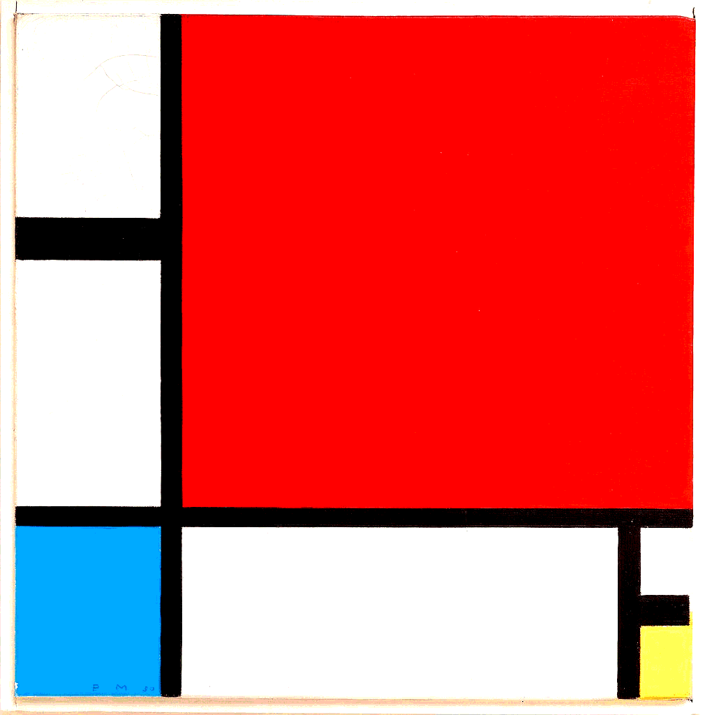
Composition II in Red, Blue, and Yellow
Piet Mondrian [Public domain]
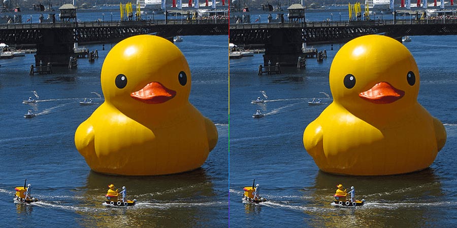
For this task, the smoothing will be disabled; this will result in sharper lines. If you are looking to disable anti-aliasing (default setting), then the noSmooth() function is what you are after. Anti-aliasing makes edges appear smoother by producing intermediate blended pixels that slightly blur the boundary.
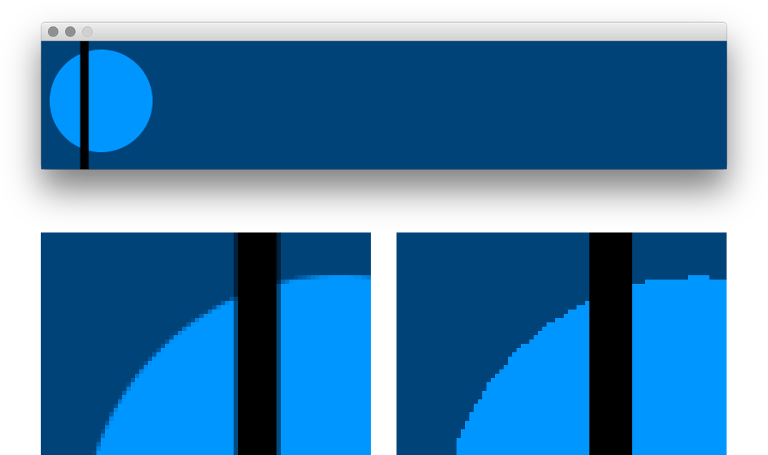
smooth() and noSmooth() on the lower-left- and right respectively.Create a new sketch and save it as “mondrian”. Copy-paste in all of the code below.
size(480,480)
background('#004477')
noSmooth()
noStroke()
'''
# red square
fill('#FF8800'); rect(0,0,width,350)
blendMode(___)
fill('#008800'); rect(0,0,width,350)

# white bottom edge
blendMode(___)
fill('#FF0000'); rect(105,350,375,130)
fill('#00BB00'); rect(105,350,375,130)
fill('#000088'); rect(105,350,375,130)

# yellow corner
blendMode(___)
fill('#FFFF00'); rect(435,0,45,height)

# white right edge squares
blendMode(___)
noStroke()
fill('#FFFFFF'); rect(435,350,45,54)
rect(0,0,105,144); rect(0,167,105,183)

# blue corner
blendMode(___)
fill('#0088FF'); rect(0,350,105,height)

# unwanted circle
blendMode(___)
fill('#0099FF'); ellipse(70,414,120,120)
# can't make the circle vanish?
# are you sure the previous blend is correct?

# thinner lines
blendMode(___)
stroke('#FFFFFF')
strokeWeight(11); line(105,0,105,height)
line(0,350,width,350); line(434,350,434,height)

strokeWeight(23)
strokeCap(SQUARE)

# thicker line upper-left
blendMode(___)
stroke('#00FFFF'); line(0,155,100,155)

# thicker line lower-right
blendMode(___)
stroke('#FFFF00'); line(440,415,width,415)
'''
You should notice that most of the code is commented out using multi-line comments. Now, moving the opening ''' down as you progress, replace each of the ___ arguments with the correct blend mode. To start you off, here’s the first solution:
# red square
fill('#FF8800'); rect(0,0,width,350)
blendMode(SUBTRACT)
fill('#008800'); rect(0,0,width,350)
'''
# white bottom edge
blendMode(___)
...
Here’s the final result for your reference.
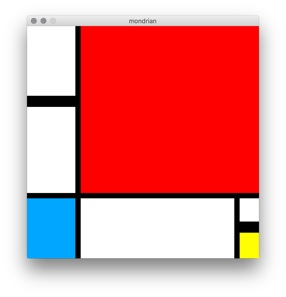
As a reminder, the blending modes are BLEND, ADD, DARKEST, DIFFERENCE, EXCLUSION, LIGHTEST, MULTIPLY, REPLACE, SCREEN, SUBTRACT.
6.6: Tint and Transparency »
Complete list of Processing.py lessons