« 1.6: Disk Space Analyser Task |
2.2: Vertices »
Lesson 1 introduced a number of 2d primitives, namely: arcs, ellipses, lines, points, quads, rectangles, and triangles. However, many shapes do not fit into any such category – like hearts (♥), stars (★), octagons, and Pikachu silhouettes, to name just a few. In this tutorial, you’ll look at drawing with points and curves, as opposed to more restrictive shape functions. Fonts also rely on curves to describe each glyph, and the latter part of this tutorial delves into Typography (and by extension, strings). Be forewarned: lesson 2 may be a little tedious, but is necessary to lay down important programming and drawing fundamentals for future lessons.
Processing deals with two types of curves: Bézier and Catmull-Rom. Both are named after the people who developed them, and both involve some complicated math. Fortunately, the complex underlying calculus is handled by Processing’s various curve functions, leaving you to deal with just the coordinates of a few control points.
Curves
The best way to grasp curves is to draw a few, then manipulate their control points. Create a new sketch and save it as “curves”. This section will be coordinate-intensive; so, to make things easier, download this “grid.png” file:
Additional sketch assets (images, fonts, and other media) always belong in a sub-folder named “data”. Create a new data folder within your curves sketch now and place the grid.png within it:
Frustratingly, many operating systems hide file extensions – that’s, the .png part of the file. However, if you dig around in your Windows or Mac Finder settings, you can get extensions to show in your file manager.
This grid will lie beneath everything you draw, assisting you in gauging x/y-coordinates. Setup your sketch using the following code:
size(500,500)
grid = loadImage('grid.png')
image(grid, 0, 0)
noFill()
strokeWeight(3)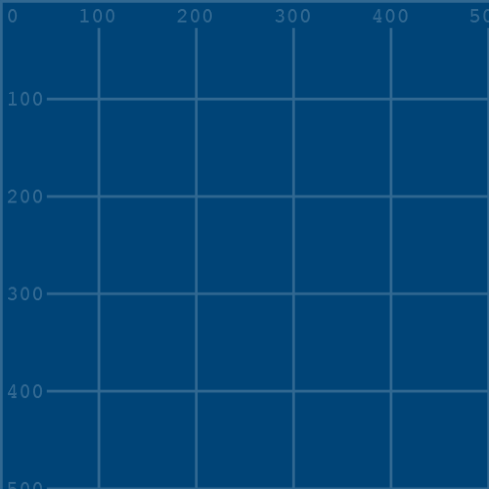
Note that it’s essential to include the file extension ('grid.png') when referencing the image file.
Catmull-Rom Splines
The Processing curve() function is an implementation of Catmull-Rom splines (named after Edwin Catmull and Raphael Rom). Once visualised, the operation of these curves is intuitive.
Add a diagonal line to your “curves” sketch:
...

stroke('#0099FF') # pale blue
line(100,100, 400,400)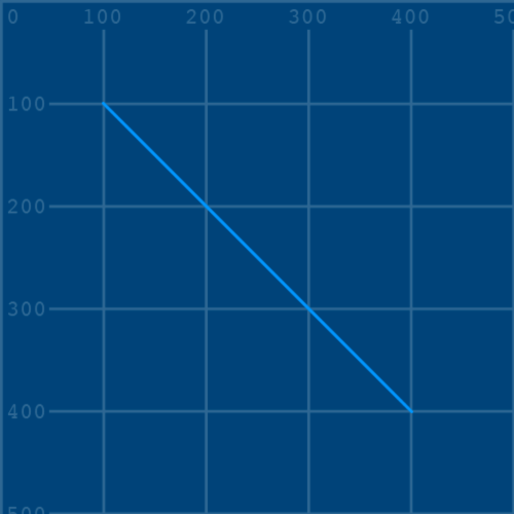
A line is drawn between the pairs of x/y coordinates specified, corresponding to the relevant lines on the grid. Now comment out the line() function and replace it with a curve():
stroke('#0099FF') # pale blue
#line(100,100, 400,400)
curve(0,0, 100,100, 400,400, 500,500)
The visual result is exactly the same. If you study the curve() arguments, you’ll notice that the four middle values match those of the line():
#line(100,100, 400,400)
curve(0,0, 100,100, 400,400, 500,500)
The extra 0,0 and 500,500 arguments represent the control point coordinates, but more on those shortly. Set the stroke to yellow and add another curve() function:
...

stroke('#0099FF') # pale blue
#line(100,100, 400,400)
curve(0,0, 100,100, 400,400, 500,500)

stroke('#FFFF00') # yellow
curve(0,250, 100,100, 400,400, 500,250)
In this instance, the control point coordinates have been tweaked – resulting in a yellow curve with a slight S-bend:
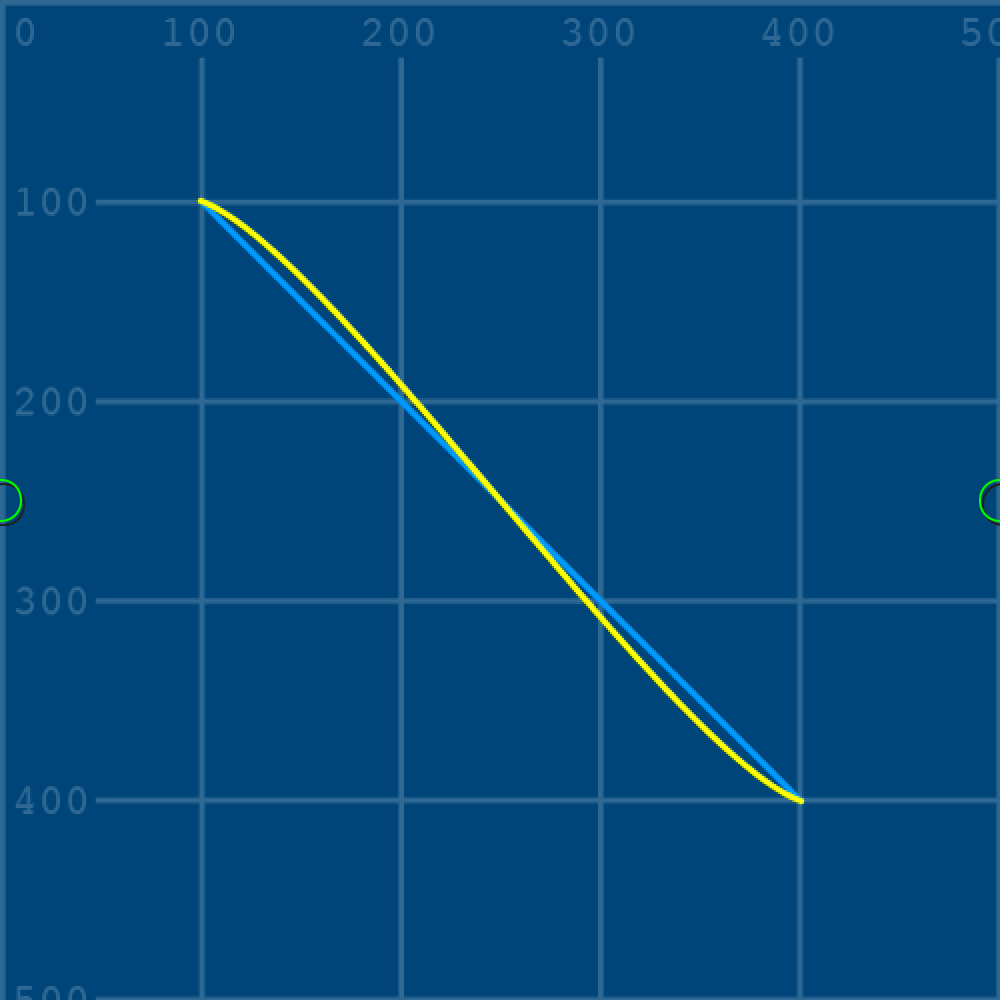
0,250) and (500,250).Now for the part where it all makes sense! To provide a clearer idea of how the control points work, add the following code:
...

stroke('#FF9900') # orange
# control point 1:
curve(0,250, 0,250, 100,100, 400,400)
# control point 2:
curve(100,100, 400,400, 500,250, 500,250)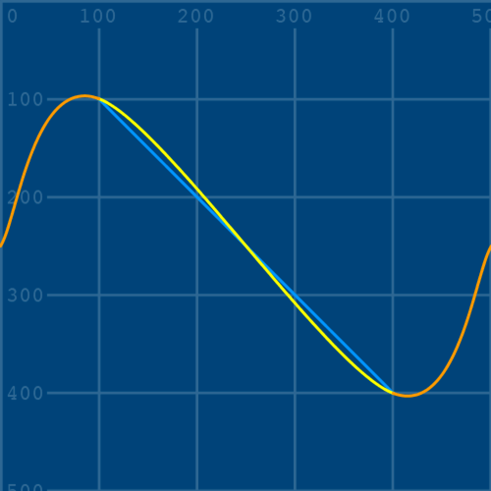
With the control point curves visualised, it should be evident how these determine the direction and amount of curvature. If you’ve ever used a flexible curve, this will look familiar. If you’re interested to know how smooth curves were ever drawn without computers, then look these up.
The curveTightness() function determines how the curve fits, as if you were replacing it with a less/more elastic material. The function accepts values ranging from -5.0 to 5.0, with 0 being the default. To experiment, add a curveTightness() line above the stroke('#FFFF00'), so as to affect all of the curves beneath it.
...
curve(0,0, 100,100, 400,400, 500,500)

curveTightness(0) # try values between -0.5 and 0.5
stroke('#FFFF00') # yellow
...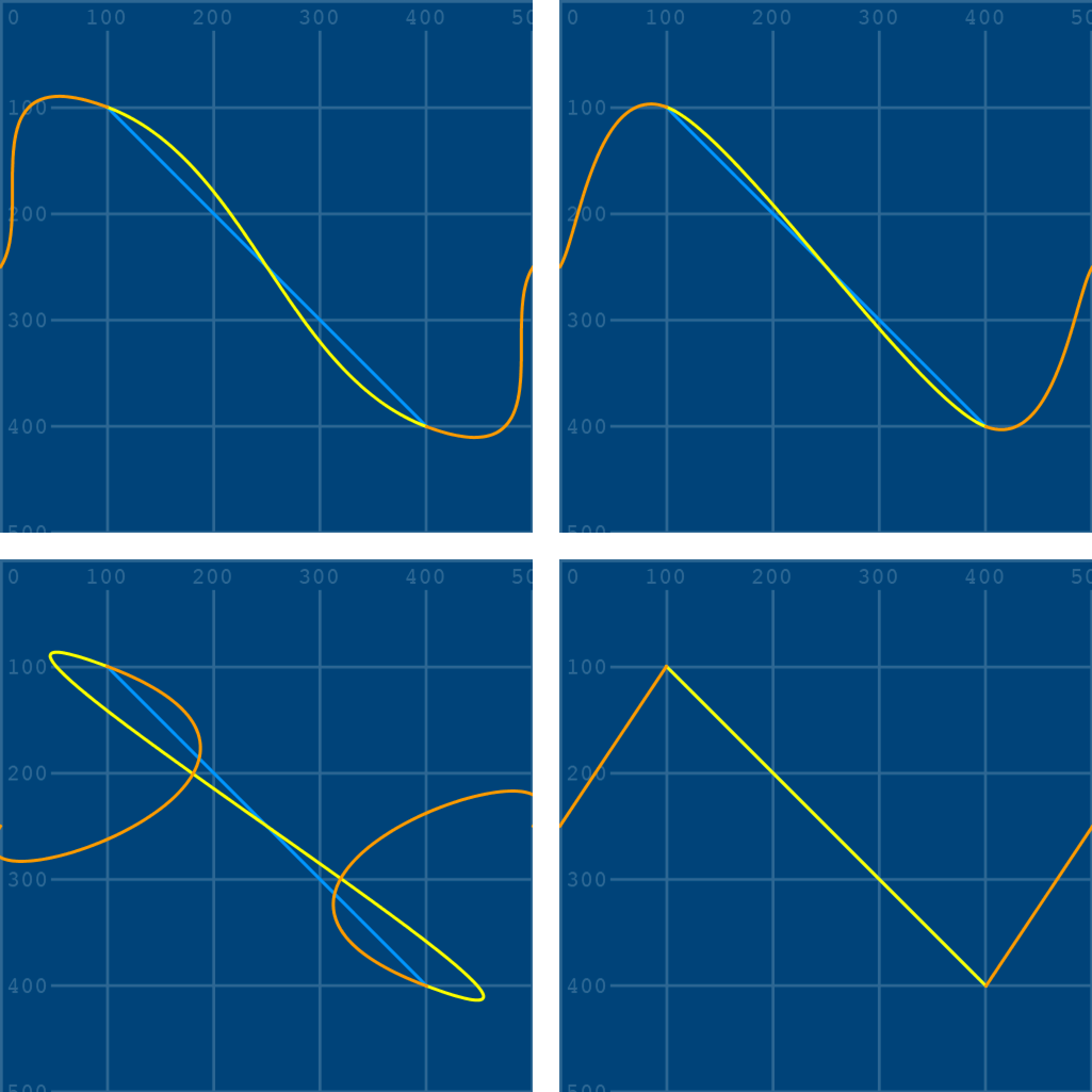
curveTightness(-1);
curveTightness(0);
curveTightness(1);
curveTightness(5).
Bézier Curves
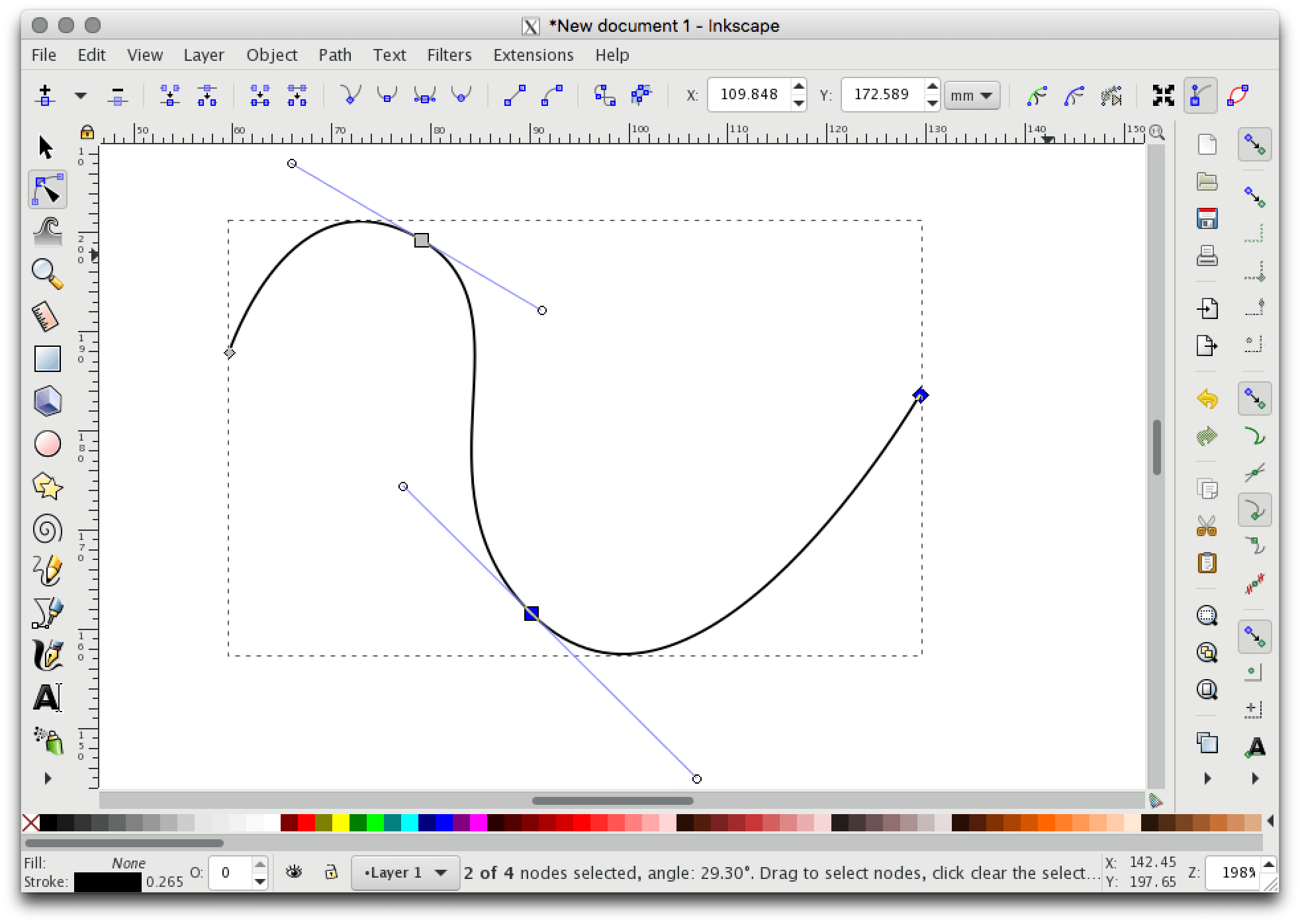
French engineer, Pierre Bézier popularised, but did not create the Bézier curve. He used them in his of design automobile bodies at Renault, devising a system whereby the shape of a curve is controlled by series of anchor and control points. If you’ve any experience with vector graphics drawing software, these will look familiar. Popular such applications include Adobe Illustrator and Inkscape, where Bézier curves are commonly referred to as “paths”.
Bézier curves are widely used in computer graphics. Their ability to model smooth curves makes them fundamental to vector graphics, animation paths, and fonts. Vector graphics (such as SVG files) can scale to any size – making them resolution-independent. Consider a digital photograph: as you zoom further and further in toward a given point, discernible squares of colour appear. Popular photographic file formats, such as JPG and PNG, are comprised of a pixel grid, the dimensions of which limit the overall resolution. However, in the case of vector-based graphics, the points along a Bézier curve can be recalculated to fit any resolution.

The bezier() function takes the following arguments, expanded across multiple lines here for easier comprehension:
bezier(
  vertex_point_1_x, vertex_point_1_y,
  control_point_1_x, control_point_1_y,
  control_point_2_x, control_point_2_y,
  vertex_point_2_x, vertex_point_2_y
)
Yikes! That’s a lot of arguments. Add some code to draw a Bézier curve, but use four variables to represent the control points:
...

stroke('#FF99FF') # pink
cp1x = 250
cp1y = 250
cp2x = 250
cp2y = 250
bezier(400,100, cp1x,cp1y, cp2x,cp2y, 100,400)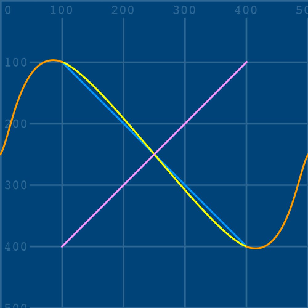
Notice how all of the cp__ variables reference the centre of the display window (250, 250), meaning that all of the control points currently lie where the yellow and pale pink lines cross. To visualise how the curve is manipulated, add a red line connecting the first vertex and control point. Adjust the cp1y variable to add some curve:
...

cp1y = 200
...
bezier(400,100, cp1x,cp1y, cp2x,cp2y, 100,400)

stroke('#FF0000') # red
line(400,100, cp1x,cp1y)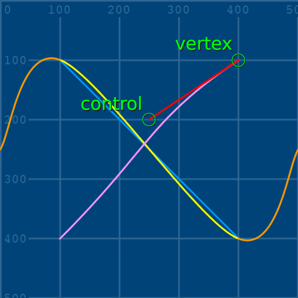
The bezier() and line() functions now share the control point’s x/y-coordinates. Making any adjustments to cp1y and cp1x, therefore, affects both functions. Add another red line to connect the lower/second vertex and control point:
...
cp2x = 320
cp2y = 350
...
bezier(400,100, cp1x,cp1y, cp2x,cp2y, 100,400)

stroke('#FF0000') # red
line(400,100, cp1x,cp1y)
line(100,400, cp2x,cp2y)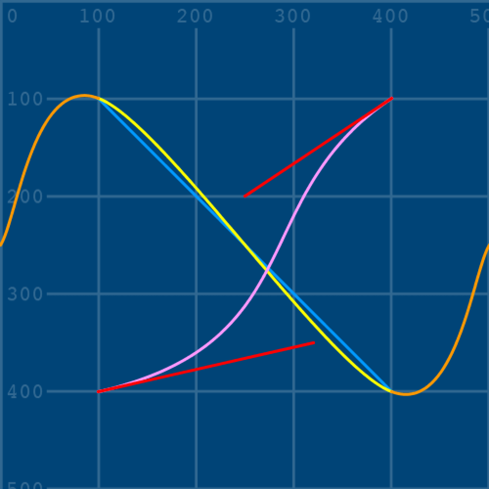
Observe how the red handles ‘magnetically’ draw the line toward the control point. Getting the hang of where to place the vertex- and control points for any desired curve takes some practice. Perhaps try the Bézier Game to hone your skills:
You can also develop your Bézier skills using Inkscape (free), Illustrator, or other similar vector graphics drawing software. It’s usually easier to draw shapes using such software, then gauge the relevant control points for Processing – which is how the tasks for this tutorial were devised ;)
2.2: Vertices »
Complete list of Processing.py lessons