« 2.1: Curves |
2.3: Strings »
Vertices
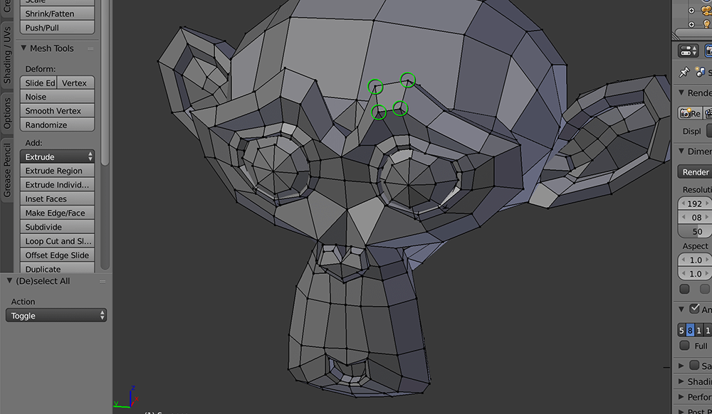
You can think of vertices as the dots in a connect-the-dots style drawing puzzle. A triangle requires three vertices; a pentagon, five; a five-pointed star (★), ten; and so forth. By connecting vertices using lines and curves, the shape possibilities become limitless. A vertex (singular) is not limited to two-dimensional space – for instance, Blender’s Suzanne (a monkey head) has around five-hundred vertices positioned in 3D space.
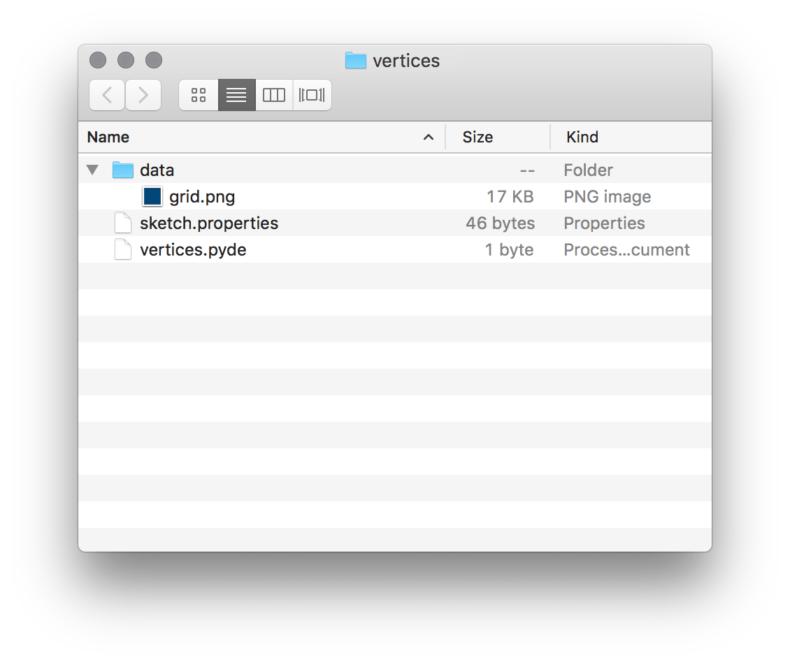
Create a new sketch and save it as “vertices”. Within the new vertices folder, add a “data” folder containing the grid.png file from your last sketch.
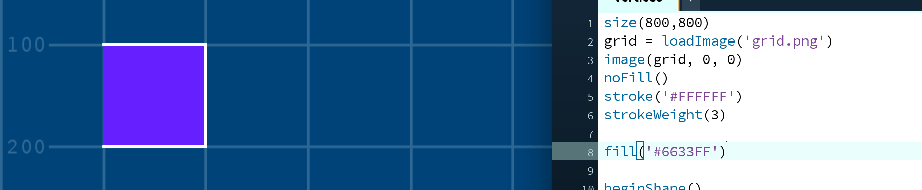
size(800,800)
grid = loadImage('grid.png')
image(grid, 0, 0)
noFill()
stroke('#FFFFFF')
strokeWeight(3)
Now draw a square using vertices:
...

beginShape() # begins recording vertices for a shape ...
vertex(100,100)
vertex(200,100)
vertex(200,200)
vertex(100,200)
endShape()   # stops recording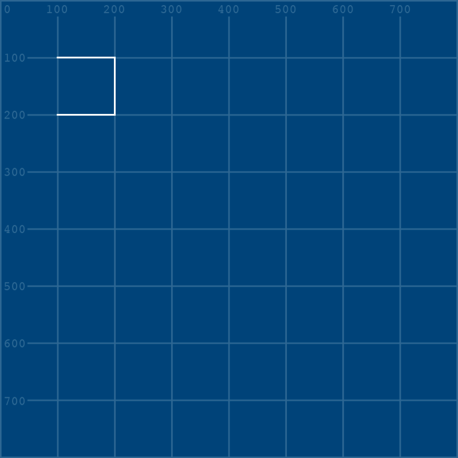
The beginShape() and endShape() functions should be self-explanatory. But, the shape will not automatically close unless you use endShape(CLOSE). However, an active fill() will fill a shape however it can:
There are also various parameters one can provide the beginShape() function to determine how the enclosed vertices are connected, if at all:
...
strokeWeight(3)

beginShape(POINTS) # begins recording vertices for a shape ...
...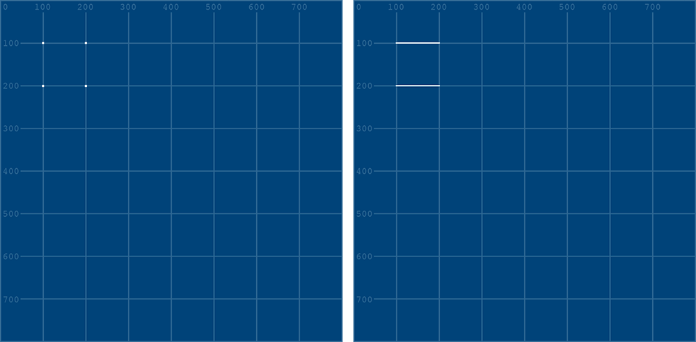
beginShape(POINTS); right: beginShape(LINES)For other beginShape() parameters, consult the reference.
Bézier Vertices
The bezierVertex() function allows one to create curved shape lines. There’s also a curveVertex() for Catmull-Rom-type curves, but lesson 2 will focus on the Bézier type, as these allow for greater control and more graceful curves.
The bezierVertex() function takes the following arguments, expanded across multiple lines here for easier comprehension:
bezierVertex(
  control_point_1_x, control_point_1_y,
  control_point_2_x, control_point_2_y,
  vertex_point_2_x, vertex_point_2_y
)
To get a better grip on how this function works, we’ll work toward completing the remaining shapes depicted below. The pale blue lines/circles provide a visual indication of where the handles and control-points lie (so there’s no need to recreate them).
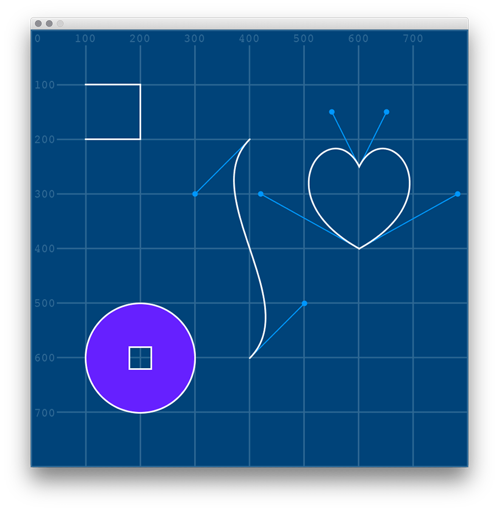
You’ll be referencing this image repeatedly through this section. It may be useful to save a copy and open a preview of it alongside your Processing editor.
S-Bend
The S-bend is comprised of two vertices, both of which are attached to control points. Of course, this is a curve, so you could draw it using a bezier() function. However, the purpose of this section is to introduce shapes. Within a beginShape(), you can mix bezierVertex(), curveVertex() and vertex() however necessary. But, the first time a bezierVertex() is used, it must be prefaced with a vertex(). Begin a new shape and place the first (in this case, upper) vertex:
...
endShape(CLOSE)

beginShape()
vertex(400,200) # starting (upper) vertex
endShape()
Now add the second vertex using bezierVertex():
...
endShape(CLOSE)

beginShape()
vertex(400,200) # starting (upper) vertex
bezierVertex(
  300,300, # control point for the starting vertex
  500,500, # control point for the second (lower) vertex
  400,600  # second (lower) vertex coordinates
)
endShape()
I’ll admit, it’s a bit confusing. But, with the positions of the vertices presented for you in the reference image, it’s really just a matter of writing in the correct sequence of coordinates.
Heart
You can think of the heart shape as two lines connecting two vertices. To begin, draw one half of the shape:
  ...
)
endShape()

beginShape()
vertex(600,400)
bezierVertex(420,300, 550,150, 600,250)
endShape()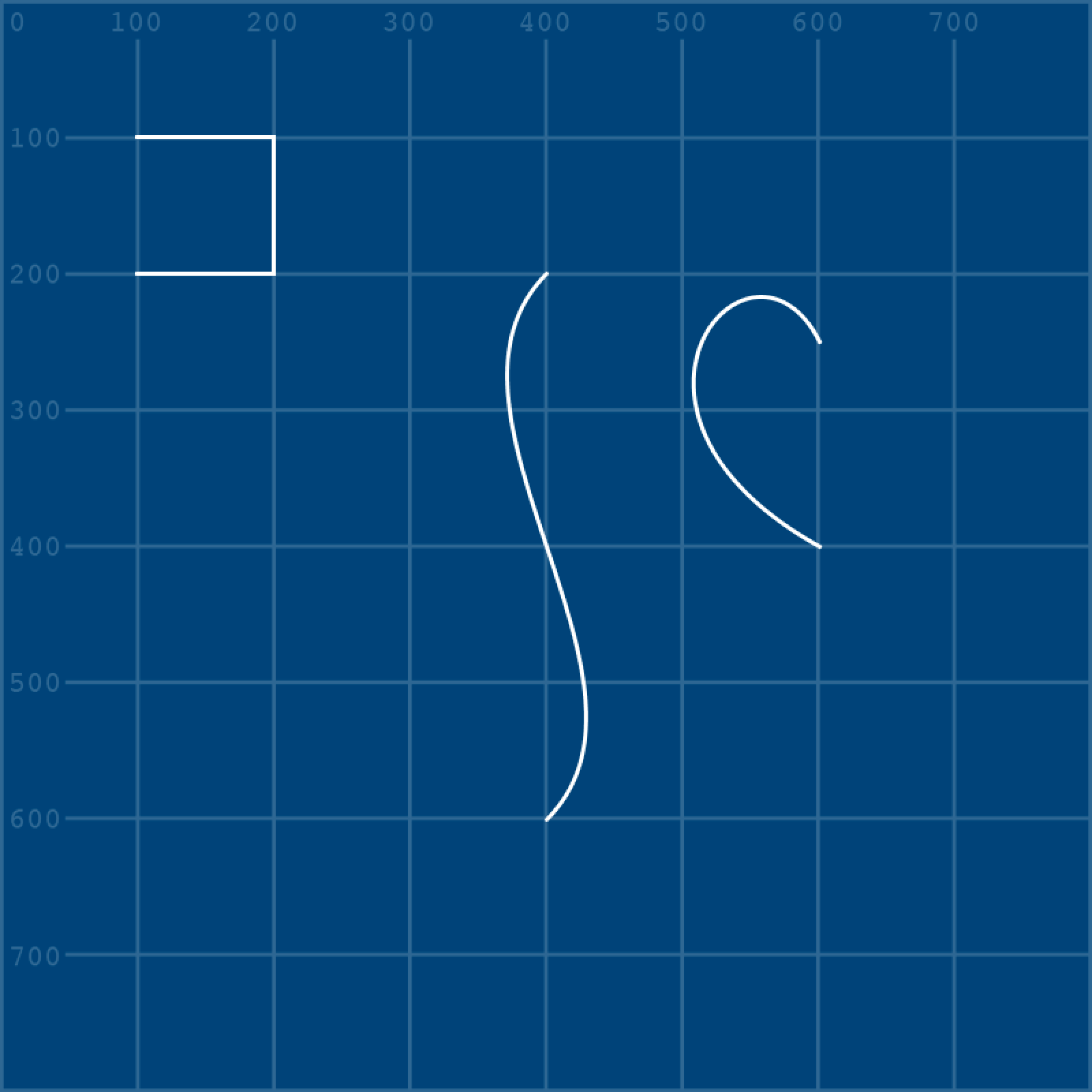
All that’s left for you to do is complete the right-half of the heart. Add a second bezierVertex() line and fill-in the arguments:
beginShape()
vertex(600,400)
bezierVertex(420,300, 550,150, 600,250)
bezierVertex(___,___, ___,___, 600,400)
endShape()
Chinese Coin
Round metal coins with square holes in the centre were first introduced in China many centuries ago. The violet-filled shape resembles such a coin, albeit with none of the relief/engraving. Its form requires that one shape be subtracted from another. Processing provides the beginContour() and endContour() functions for this purpose.
The first challenge is the outer circle. The contour functions are used within a beginShape() and endShape(), so using an ellipse function is not an option. However, circles can be drawn using Bézier curves:
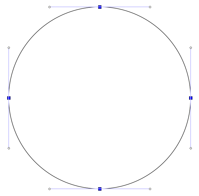
You can begin by forming a circle using a diamond shape:
...

beginShape()
vertex(100,600)
vertex(200,500)
vertex(300,600)
vertex(200,700)
vertex(100,600)
endShape()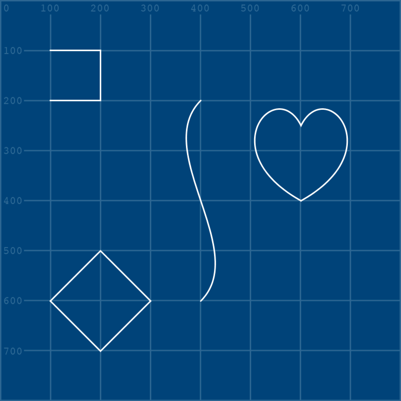
With your vertices in place, you can now convert the vertex() functions to bezierVertex() functions. Remember, though: the first point must be a vertex().
...

beginShape()
vertex(100,600)
bezierVertex(___,___, ___,___, 200,500) # vertex(200,500)
bezierVertex(___,___, ___,___, 300,600) # vertex(300,600)
bezierVertex(___,___, ___,___, 200,700) # vertex(200,700)
bezierVertex(___,___, ___,___, 100,600) # vertex(100,600)
endShape()
To save you having to workout where the control points lie, here are the missing arguments:
bezierVertex(100,545, 145,500, 200,500)
bezierVertex(255,500, 300,545, 300,600)
bezierVertex(300,655, 255,700, 200,700)
bezierVertex(145,700, 100,655, 100,600)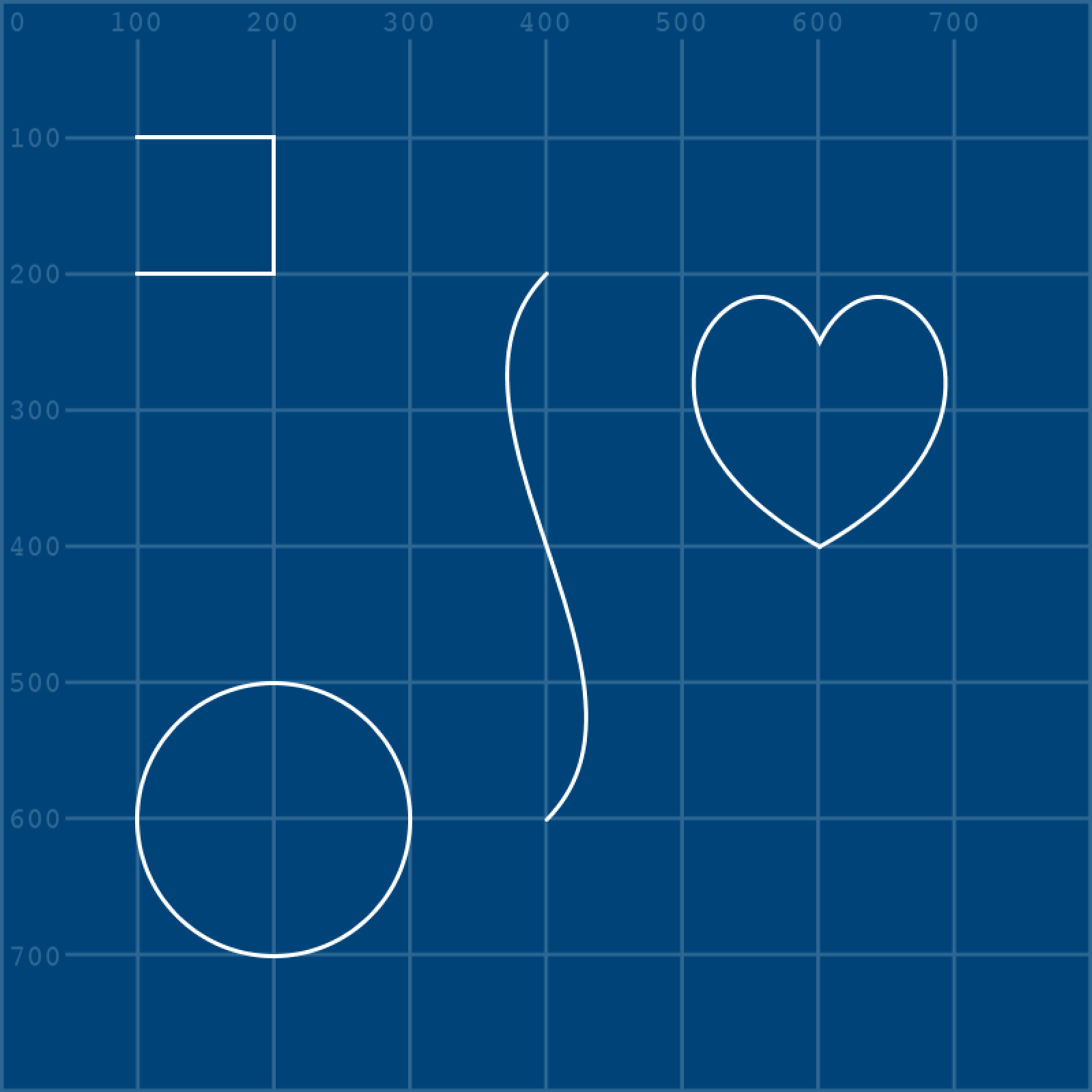
With the circle in place, you can go about removing a square from the middle. This is a relatively straightforward exercise, but there’s one crucial thing to be aware of: one must use reverse winding for the subtracted shape. Read through the circle code again and notice how all of the vertices are plotted in a clockwise manner; this means that the square’s vertices must be plotted counter-clockwise, i.e. opposite to the winding of the shape from which it will subtract.
Place the square’s vertices within a beginContour() and endContour() function. Of course, you cannot observe the effect unless you add a fill:
fill('#6633FF')
beginShape()
vertex(100,600)
bezierVertex(100,545, 145,500, 200,500)
bezierVertex(255,500, 300,545, 300,600)
bezierVertex(300,655, 255,700, 200,700)
bezierVertex(145,700, 100,655, 100,600)
beginContour()
vertex(180,580)
vertex(180,620)
vertex(220,620)
vertex(220,580)
endContour()
endShape()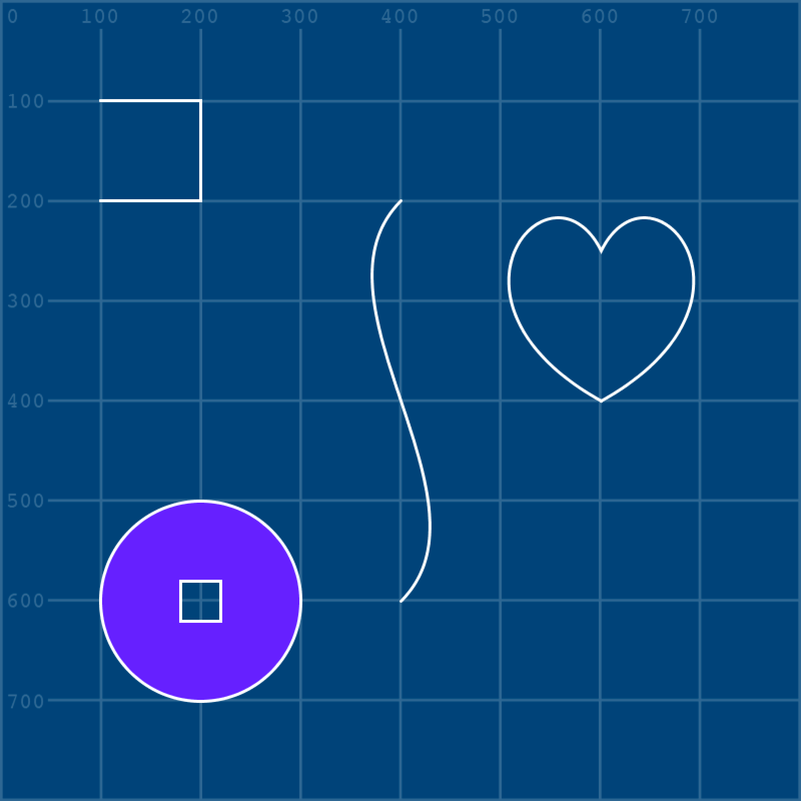
Bézier Task
Time for a challenge!
Create a new sketch and save it as “bezier_task”. Within the sketch’s folder, create a “data” sub-folder and add a copy of the grid.png, along well as this image file:
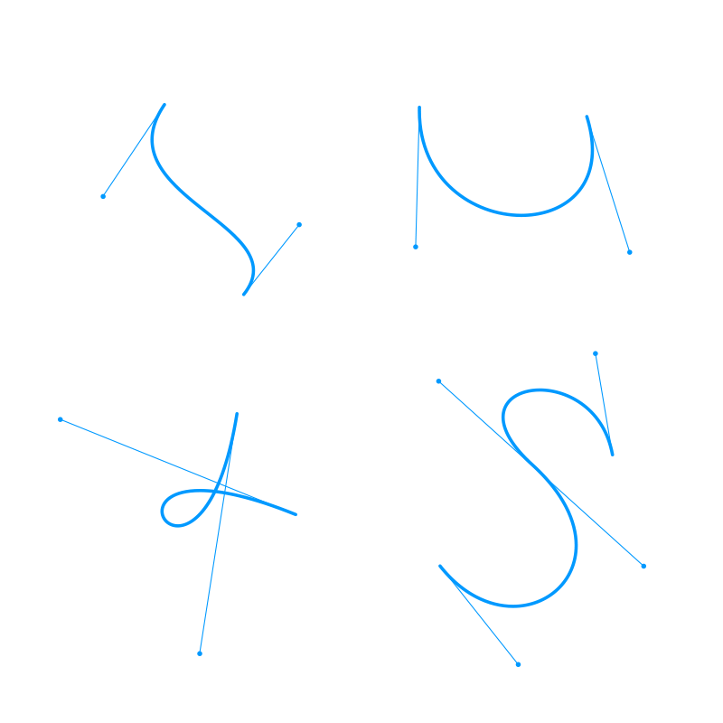
Add the following setup code:
size(800,800)
grid = loadImage('grid.png')
beziers = loadImage('beziers.png')
image(grid, 0, 0)
image(beziers, 0, 0)
noFill()
stroke('#FFFFFF')
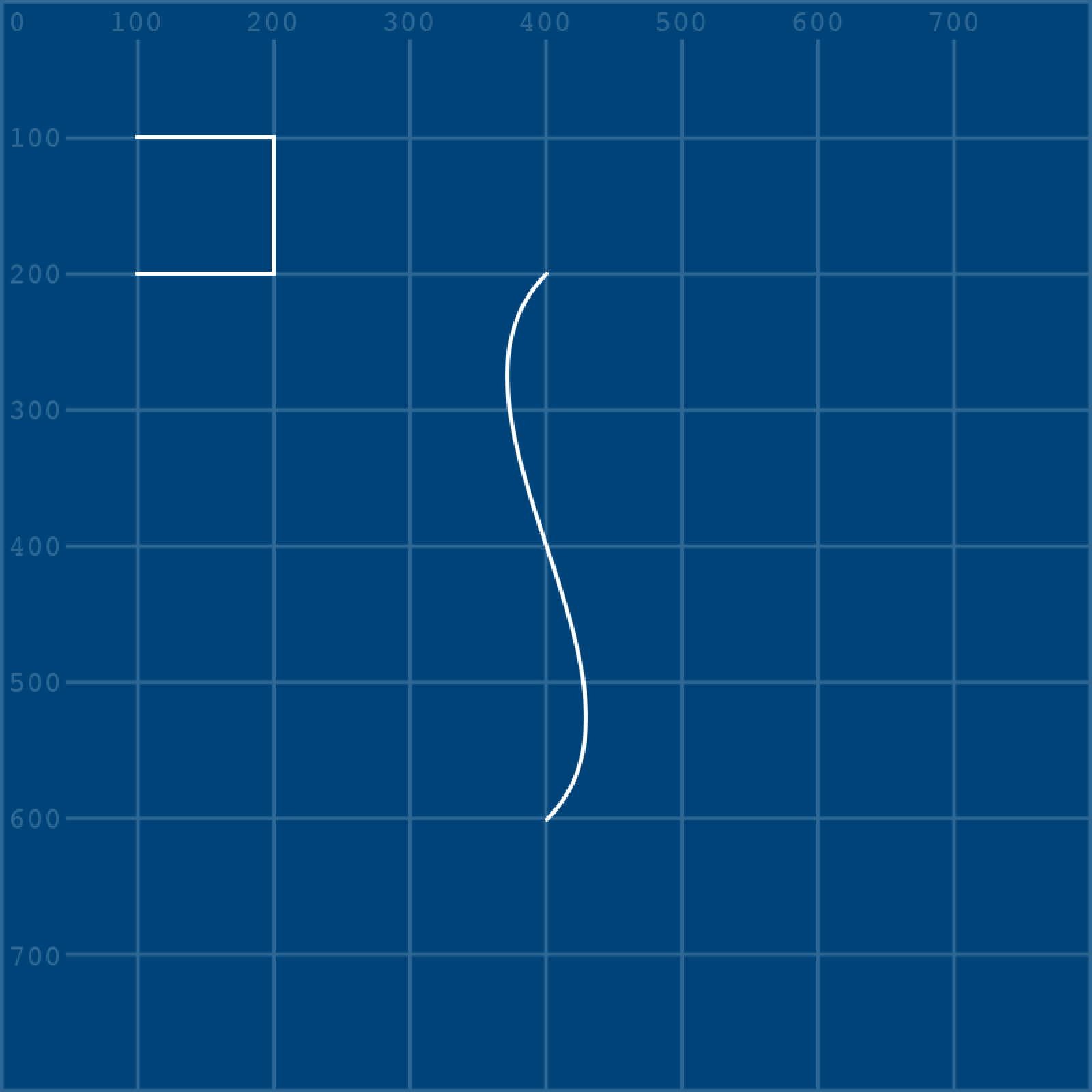
strokeWeight(3)When you run the sketch, you’ll see four Bézier curves. Recreate them using bezierVertex().
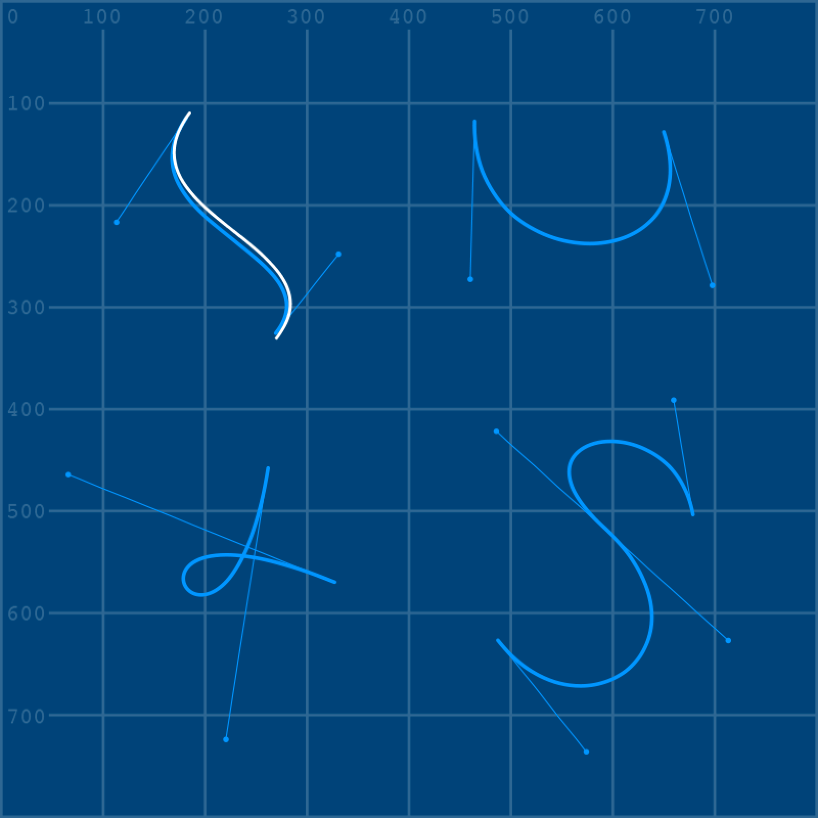
The curves need not be pixel-perfect replicas, as this is just something to get you used to working with them.
2.3: Strings »
Complete list of Processing.py lessons