« 7.3: Keyboard Interaction |
7.5: ControlP5 »
Collision Detection
To establish if two or more shapes have intersected within a game, one performs collision detection tests. There are many algorithms for this – the more accurate types, though, are more demanding on your system (and coding skills). We’ll look at one of the most basic forms of collision detection techniques, namely, axis-aligned bounding boxes (or AABBs).
With AABB collision testing, a rectangular bounding box encapsulates each collide-able element. Of course, many games assets are not perfectly rectangular, so one must sacrifice some accuracy.
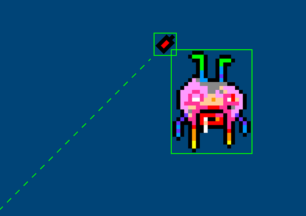
We can attempt to improve the perceived accuracy by shrinking the bounding box, using multiple boxes, or employing a different yet comparably performant shape – like, a circle. You could even combine bounding- boxes and circles. Be aware, though, that each obstacle, item, and enemy on screen is tested for collisions with every other obstacle, item, and enemy. Complex bounding volumes can cause a significant increase in processing overhead, and as a result, slow or jerky performance.
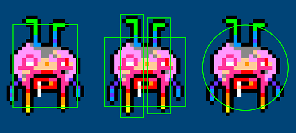
In a few chapters time, we’ll take a look at circular collision volumes. For even greater accuracy, there are polygonal bounding volumes that can accommodate just about any shape, but these require a heap of involved math!
To begin with AABBs, add a collectable item – a red square – to the stage:
def draw():
    ...
    itemx = 300
    itemy = 60
    fill('#FF0000')
    rect(itemx, itemy, 10, 10) # red item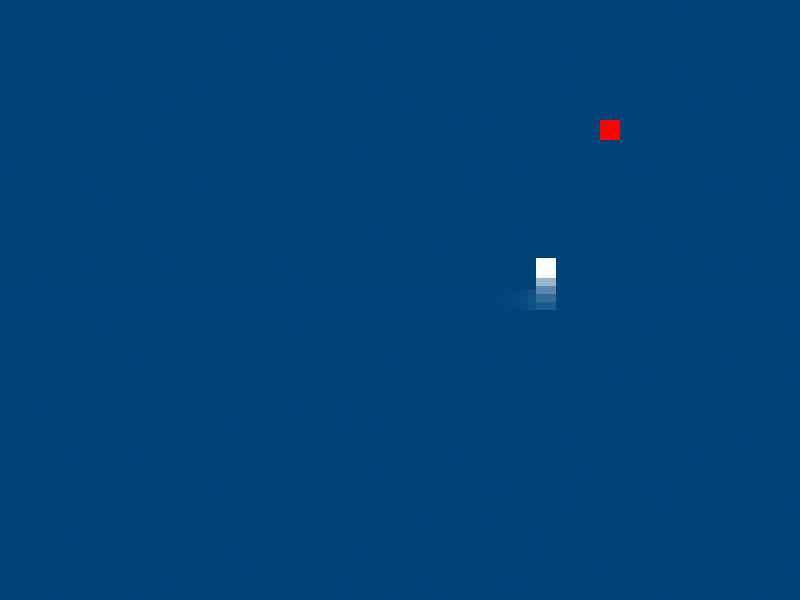
The collision test will be handled using a single if statement and we’ll build-up the conditional expression one piece at a time. The snake’s trail will not trigger any collisions, just the solid white square at its ‘head’. Add a new if statement to the draw() function:
...
rect(itemx, itemy, 10, 10) # red item
if (
playerx+10 >= itemx
):
fill('#00FF00')
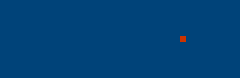
text('hit!', 373,28)If part of the head is anywhere to the right of the red square, a hit’s registered. The rect() draws squares from the top-left corner across-and-down, so it’s necessary to use x+10 (the x-coordinate plus the width of the head) to ascertain the x-coordinate of the head’s right edge. Run the sketch to confirm that this is working. Watch for the “HIT!” that appears in the top-left corner of the display window. The shaded green area in the image below highlights the ‘collision’ zone as it operates currently.

To refine this further, expand on the condition to test whether the player has ventured too far rightwards to trigger any possible collision.
    ...
    rect(itemx, itemy, 10, 10) # red item

    if (
          playerx+10 >= itemx and playerx <= itemx+10
       ):
        fill('#00FF00')
        text('hit!', 373,28)
To explain:
playerx+10 >= itemx
checks if the right edge of the head is overlapping the left edge of the red item;
playerx <= itemx+10
checks if the left edge of the head is overlapping the right edge of the red item.
This constrains the hit-zone to a vertical band as wide as the item.
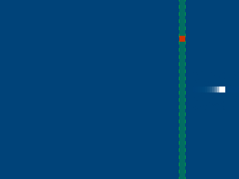
The head no longer registers a hit once it has passed the right edge of the item. However, as indicated by the green area in the image, anywhere directly above or below the item reports a collision. To resolve this, add additional checks for the y-axis.
    ...
    rect(itemx, itemy, 10, 10) # red item

    if (
         playerx+10 >= itemx and playerx <= itemx+10
     and playery+10 >= itemy and playery <= itemy+10
       ):
        fill('#00FF00')
        text('hit!', 373,28)
The result is an axis-aligned bounding-box that conforms perfectly to the red item.
The collision detection is now functioning correctly. From here, you could make the item disappear and apply power-up. For example, perhaps the snake’s speed could increase when upon collecting the red square? Then maybe after a short period, a new item could appear at some random new location? Before you begin trying anything, though, let’s look at one another important game programming concept: delta time.
Delta Time
Films run at a constant frame rate. Games attempt to run at a constant frame rate, yet there’s often fluctuation. Your Sna game is ticking over at 30 fps, as specified in the setup function. Your computer is powerful enough to check for key input, render the snake’s new position, and detect possible collisions – each and every frame – without producing any noticeable lag. However, there are instances where a game must perform many additional interframe computations. For example, there may be twenty collectable items scattered about the stage; in such a scenario, a further nineteen AABB collision tests must take place before a new frame can be displayed. More likely, though, it would take thousands of collision tests per frame to produce any perceivable slow-down.
Edit the yspeed variable so that the snake immediately heads upward when the sketch runs. In addition to this edit, add an if statement to the bottom of your draw function to record the total milliseconds elapsed upon the snake reaching the top edge.
...
yspeed = -2

def draw():
    ...
    if playery > 145:
        fill('#00FF00')
        text(millis(), width/2,28)
        noLoop()
The if statement detects when the snake is somewhere below its starting position. In other words, just as the head teleports to the lower half of the stage, but before rendering it at the opposite edge.
Run the sketch. The snake heads-off as soon as the display window opens. Upon reaching the top-edge, the noLoop() halts everything and the millisecond count is displayed.

The fastest possible time that the snake can reach the boundary is 2500 milliseconds. My computer managed 2833 milliseconds, but your system could be slower or faster. The snake has 300 ÷ 2 = 150 pixels to cover, travelling at a speed of 2 pixels-per-frame. So, that’s 150 pixels ÷ 2 pixels-per-frame = 75 frames to reach the edge. Recall that the game is running at 30 frames per second. Therefore, 75 total frames ÷ 30 fps = 2.5 seconds, or, 2500 milliseconds. Why can’t it manage 2500 milliseconds flat? Well, the very first frame takes some extra time because Processing needs to setup a few things.
To measure the time elapsed between the drawing of each new frame, add the following code:
...
lastframe = 0

def draw():
    global currframe, lastframe
    currframe = millis()
    deltatime = currframe - lastframe
    print(deltatime)

    ...

    lastframe = currframe
The currframe variable is used to record the current time – which can then compared with the lastframe variable. The difference between these two values is assigned to the deltatime variable. Run the sketch. Once the snake has reached the top edge, scroll back up through the Console output. The deltatime averages around 33 milliseconds – because 1000 milliseconds divided by 30 (the frame rate) is 33.3 recurring. The exception is the very first value, as the first frame takes significantly longer to process.
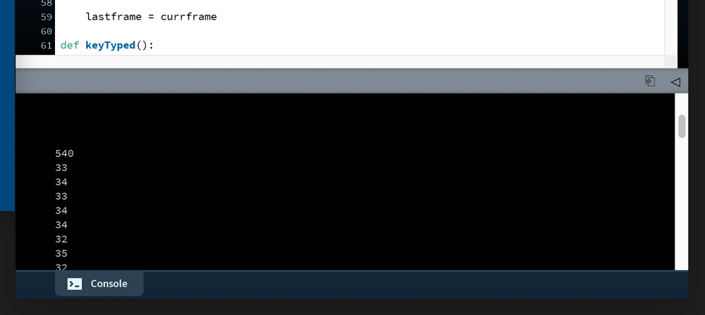
deltatime averages around 33 milliseconds, but the first value is much larger.To emulate some heavier processing loads, as if there were thousands of collisions to test, add a highly demanding (if pointless) computational task to the end of your draw loop just before the lastframe = currentframe line:
def draw():
    ...
    for i in range(ceil(random( 900 ))):
            for j in range(i):
                atan(12345*i) * tan(67890*i)

    lastframe = currentframe
This new for loop does nothing useful. It performs a bunch of intense trigonometry calculations only to discard the values when complete. All of this extra trig-crunching should slow things down. Run the sketch to see what happens.

You should experience a noticeable reduction in frame rate. Note, however, that the loop employs a random function. The lag effect is, hence, erratic as the loop may run anywhere between zero and 900 times in a single draw. In other words, the snake will move smoothly, but then randomly struggle before speeding up again. My computer clocked 5985 milliseconds for the boundary sprint, but yours could be much slower or faster. If you find that your computer is grinding to a near-halt, reduce the 900 to something a bit more manageable. Conversely, if everything seems to be running about as smoothly as before, try doubling this value. You’ll want to find some number that, roughly speaking, halves the snake’s average speed.
You’ll also notice that the deltatime (the milliseconds elapsed between each frame) values are now far more erratic and generally larger.
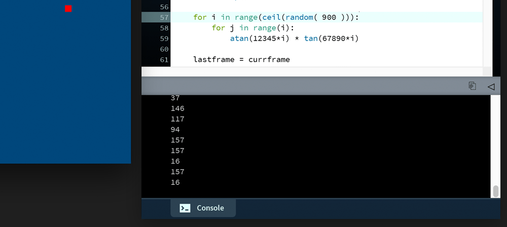
deltatime values are larger and more erratic.This is where the delta time proves useful. The time between frames can be used to calculate where the snake’s head should be, as opposed to where it managed to reach. To calculate the projected playery position, multiply it by deltatime divided by the required frame interval (33.3 milliseconds).
    ...
    playery += yspeed * (deltatime/33.3)
    ...
Run the sketch. The snake reaches the top-edge in around 2500 milliseconds, even slightly under, as if there were no lag at all. However, rather than rendering each successive head two-pixels apart, the head ‘leaps’ in larger, unevenly-sized increments. The size of each leap is dependant on how much time is required to catch up. This results in a longer trail, as the starting position in now fewer frames from the ending position. Moreover, some discernible gaps may appear in the trail, although this will depend on how much your system struggles to match 30 frames per second.

You can now adjust the loop’s 900 value as you wish and the snake still reaches the top edge in around 2500 milliseconds (give or take a few hundred).
Delta time, thus, helps maintain a constant game speed despite variations in frame rate. We are ‘dropping’ frames to keep apace, but, ultimately, delta time helps smooth out the movement values. It can also be used to limit frame rates in cases where a game may run too fast. Generally speaking, the motions of any positioning, rotation, and scaling operations should incorporate delta time. On the other hand, games can behave very strangely if physics calculations mix with variable frame rates. Many game engines, hence, include fixed- and variable time-step functions – like draw() – to separate out physics and graphics code.
If you wish to move the player around freely again, be sure to remove the if playery > 145 code.
that’s as deep as we’ll venture into game development concepts. If it’s games you are serious about, then you’ll need to explore further using other resources. That said, the concepts and techniques covered in the previous and upcoming tutorials are integral to any journey towards game development.
7.5: ControlP5 »
Complete list of Processing.py lessons