In this final part, you’ll learn some Blender scripting techniques—like how to address, manipulate, copy, and animate mesh primitives using code. To combine all of those techniques, you’ll create a wavy pattern of cones—a cool-looking animation that you can convert into a looping GIF.
I’ll review the all-important bpy library using a selection of attributes and methods from the bpy.data module. I’ll also touch on how to import code from other Python files, as well as using other code editors to write your Blender code. Of course, there’s plenty more to creative coding with Blender, but that’s all I cover in this short series of tutorials.
Before proceeding, launch Blender (using the command line). If you have it open already, create a new Blender file using File > New > General. You’re looking at a new scene with a cube located at an x-y-z coordinate of (0, 0, 0).
Importing bpy
The bpy library is what makes all of the magic happen. It contains nine main modules that enable you to control Blender using Python; those are bpy.app, bpy.context, bpy.data, bpy.msgbus, bpy.ops, bpy.path, bpy.props, bpy.types, and bpy.utils. In the Python Console, the bpy library is automatically imported and available to use immediately. But when you’re writing Python scripts in the Text Editor (or any other code editor), you must add the necessary import line(s) before you can utilise bpy.
NOTE: In addition to
bpy, Blender includes several standalone modules, likeaudfor audio, andmathutilsfor manipulating matrices, eulers, quaternions and vectors.
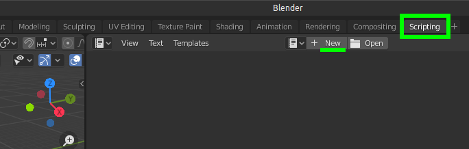
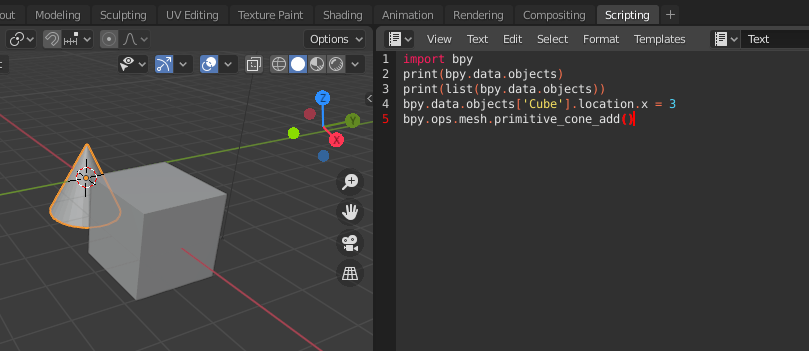
Switch to the Scripting tab (Figure 3.1), then click New in the Text Editor to create a new Python script.
Add the following lines to your new script to import bpy and print a list of the objects in your scene:
import bpy
print(bpy.data.objects)
Run the script (using Alt-P or the ▶ button). Your terminal should display:
<bpy_collection[3], BlendDataObjects>
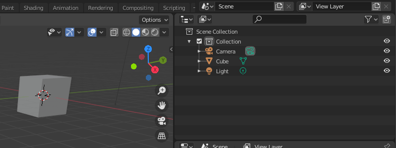
Recall that the bpy_collection[3] part indicates there are three objects—a camera, cube, and a light (Figure 3.2). If you added or removed anything from the scene, the [3] changes to reflect the total number of objects.
But there’s much more you can do with bpy.data.objects. For instance, you can use it to address specific items in the Outliner listing.
Addressing Objects
In part 2, you used the Python Console to affect the object selected in the 3D Viewport. More often, though, you’ll want to address objects via Python scripts without relying on what’s selected in the GUI. You can use bpy to select objects by name, their position in a sequence of objects, or some other property. If you’re using bpy.context, you must select the cube in the 3D Viewport (so it’s outlined orange) to manipulate it with Python code. With bpy.data.objects, you can address an object regardless of what’s active in the Blender interface.
Use the Python list() function with bpy.data.objects to print a list of the objects in your scene:
print(list(bpy.data.objects))When you run the script, it should display the following output in the terminal:
[bpy.data.objects['Camera'], bpy.data.objects['Cube'], bpy.data.objects['Light']]
You can address any object using its key (item name) or index (order in the sequence). Index values begin at zero—so Camera is item 0, Cube is item 1, and so forth. You can use bpy.data.objects['Cube'] or bpy.data.objects[1] to address the cube. Next, you’ll manipulate the cube using different attributes and methods.
Attributes and Methods
If you’re familiar with any object-oriented programming language, you’ve encountered attributes and methods before (and you’ve likely identified a few examples of these in the code so far). I won’t review every attribute and method in the Blender scripting API—there are far too many for that! Instead, I’ll use a few examples to help you discover what’s available; you can use the API documentation for the rest.
Attributes
Attributes are like variables that belong to objects. An object’s data type determines its attributes. For instance, a cube—a three-dimensional mesh, composed of vertices—includes attributes for its dimensions, coordinates, and so on. The cube data type is bpy_types.Object; you can confirm this by printing type(bpy.data.objects['Cube']) in the terminal or console.
The location attribute—one of the many bpy_types.Object attributes—contains the coordinates for your cube, that you can use to reposition it:
bpy.data.objects['Cube'].location = (3, 0, 0)This positions the cube at the x-y-z coordinates (3, 0, 0). In this case, you’re only affecting the x-coordinate, so instead, you might use:
bpy.data.objects['Cube'].location[0] = 3Note that .location[0] is the index of the first (x) value in (3, 0, 0). Alternatively, you can try the .location.x attribute, which is arguably the most intuitive version to read:
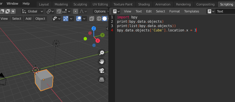
bpy.data.objects['Cube'].location.x = 3Run the script and the cube should move to its new position (Figure 3.3), three units away from the centre of the scene along the x-axis:
You’ve enabled python tooltips, so if you hover your mouse pointer over any fields in the Object Properties panel, there’s a tooltip to indicate how you address that specific attribute for that particular object in Python. This panel is usually located in the lower-right area of the Blender interface, in both the Layout and Scripting workspaces. In Figure 3.4, the tooltip reveals the Python details for the cube’s x-coordinate:
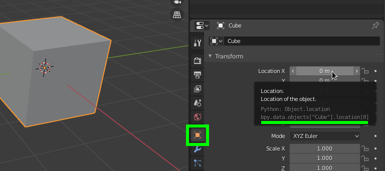
bpy.data.objects["Cube"].location[0]If you right-click on this field, there’s a menu option named Online Python Reference that opens the relevant documentation for the location attribute in your web browser (Figure 3.5).
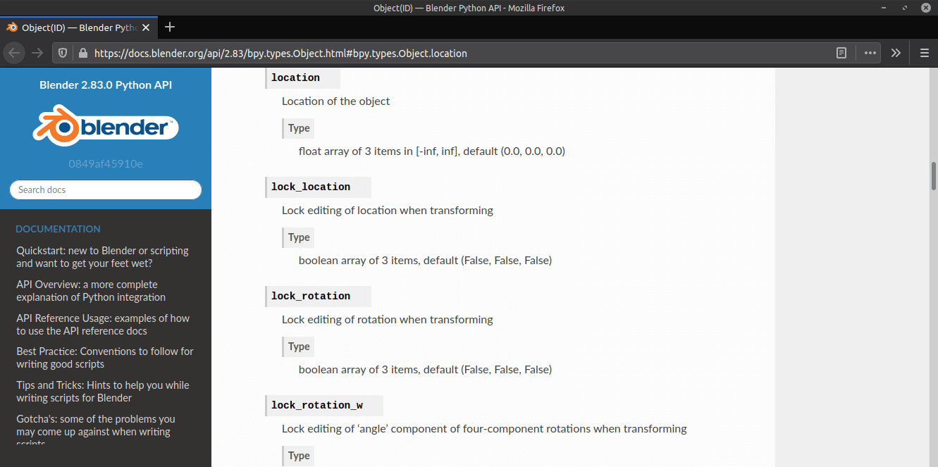
location entry in the online referenceTake note of the URL in the browser address bar: https://docs.blender.org/api/2.83/bpy.types.Object.html#bpy.types.Object.location. Specifically, everything after the last slash. There’s /bpy.types.Object.html to load the web page, followed by #bpy.types.Object.location to jump/scroll to the location entry. You can also navigate the reference using the search feature and links in the left column. Sometimes it’s handy to use your web browser search function (Ctrl+F or Cmd+F) to find something on a given page quickly. If you’d like to experiment with another attribute, perhaps try scale.
Now that you’ve used a few different attributes, let’s look at methods.
Methods
Methods are like functions that belong to objects. They perform operations—for instance, the bpy.ops.mesh module includes several methods for creating new meshes. You can easily discern a method from an attribute, because a method has a pair of parentheses on the end of it. In this section, you’ll use different methods to add and remove objects in your scene.
The primitive_cone_add() will “construct a conic mesh”; in other words, you use this method to add cones to your scene (Figure 3.6). Add this new line to the end of your script:
bpy.ops.mesh.primitive_cone_add()This should add a new cone when you run the code.
primitive_cone_add()The primitive_cone_add() method can also accept arguments to specify the cone radius, depth, location, rotation, scale, and more. Add a second cone line to your script that includes an argument to control its location:
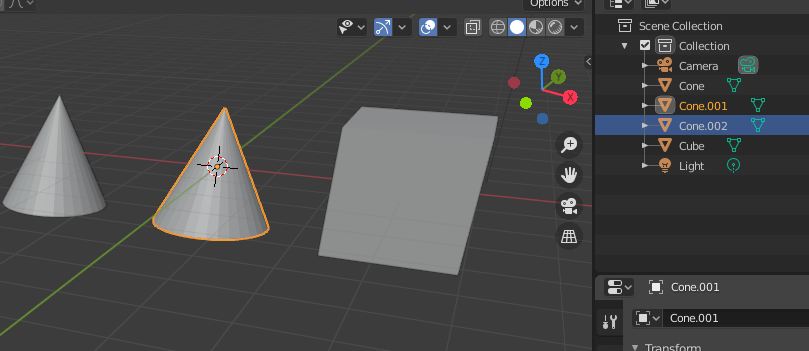
bpy.ops.mesh.primitive_cone_add(location=(-3, 0, 0))When you run the script, a new cone appears. But, if you check the Outliner panel (Figure 3.7), you’ll notice there are now three cones in the scene. The extra cone is a duplicate of the one in the centre of the stage (the same size, in the same position). Each time you run the script you’re adding further duplicates!
To prevent this duplication from occurring, you can add a loop that checks for- and removes any meshes. You don’t need the cube or its code anymore, so it’s fine that you don’t replace it. The final script looks like this:
import bpy

# clear meshes in the scene
for obj in bpy.data.objects:
    if obj.type == 'MESH':
        bpy.data.objects.remove(obj)

# add two cones
bpy.ops.mesh.primitive_cone_add()
bpy.ops.mesh.primitive_cone_add(location=(-3, 0, 0))
The remove() method removes the object (supplied in the parentheses) from the scene. Now, each time you run the script, it clears out the meshes before adding them again.
You can find many more bpy.ops.mesh methods in the API documentation.
Animation
Programming animations in Blender is immensely satisfying. You can create stunning moving images that combine the Python API, a powerful renderer, and simulation features. Bear in mind that this isn’t a ‘real-time rendering’ approach. You’ll define your keyframes up-front and render them out completely to produce a sequence of frames that form an animation. This isn’t interactive, like something you might create in Processing or some game engine. What follows is an elementary example to get you started with multi-frame programming, that builds on your existing script.
NOTE: Blender once included a game engine, a feature that has since been discontinued. However, UPBGE (a fork of the old Blender game engine project) and Armory now aim to provide complete game development solutions within the Blender environment.
Add the following code to the end of your script:
...
# animation variables
total_frames = 100
keyframe_interval = 10

# define a one hundred frame timeline
bpy.context.scene.frame_end = total_frames
bpy.context.scene.frame_start = 0

# add keyframes
for frame in range(0, total_frames + 1, keyframe_interval):
    bpy.context.scene.frame_set(frame)
    cone = bpy.data.objects['Cone']
    cone.location.x = frame / 25
    cone.keyframe_insert(data_path='location')
There are comment lines (starting with a #) to help explain each step. The for loop inserts a new keyframe every 10 frames (keyframe_interval), across a timeline that spans from frame 0 to frame 100 (total_frames). The cone advances 0.04 units along the x-axis between keyframes; Blender will interpolate/tween this movement to smooth it out.
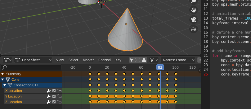
To help visualise how what’s happening, I’ve switched out the Console panel (in the area below the 3D Viewport) for the Dope Sheet. You can see each keyframe represented as a yellow dot (Figure 3.8). You press the space key to start and stop the animation; the position of the blue playhead line indicates which frame is playing.
NOTE: When you start the animation using the space key, it'll loop when it reaches the end. It's handy to leave it looping while you code so that when you rerun the script, the animation automatically refreshes the preview.
You can decide how small or large the keyframe intervals should be. By default, the movement between keyframes is linear—so, really, this animation only requires a keyframe on frames 0 and 100. But I wanted to demonstrate how you can add many more keyframes using a loop. If you wish to tweak the animation curves, you can do so using the Graph Editor.
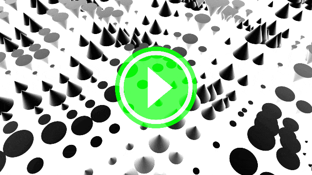
Wavy Cones (or Cony Waves?)
Here’s a script that combines all of the techniques in this tutorial to generate a wavy pattern of made of cones. Click on the image below (Figure 3.9) to view the result you are working toward:
Here’s the code for the animation:
import bpy
from math import sin, tau
# clear meshes in the scene
for obj in bpy.data.objects:
if obj.type == 'MESH':
bpy.data.objects.remove(obj)
# animation variables
total_frames = 150
theta = 0.0
# define a one hundred frame timeline
bpy.context.scene.frame_end = total_frames
bpy.context.scene.frame_start = 0
for x in range(30):
# generate a grid of cones
for y in range(30):
cone = bpy.ops.mesh.primitive_cone_add()
cone = bpy.context.object
cone.name = 'Cone-{}-{}'.format(x, y)
cone.location[0] = x * 2
cone.location[1] = y * 2
# add keyframes to each cone
for frame in range(0, total_frames):
bpy.context.scene.frame_set(frame)
cone.location.z = sin(theta + x) * 2 - 1
cone.keyframe_insert(data_path='location')
scale = sin(theta + y)
cone.scale = (scale, scale, scale)
cone.keyframe_insert(data_path='scale')
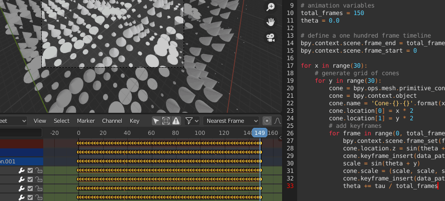
theta += tau / total_framesIn this instance, I haven’t used a keyframe interval. As the Dope Sheet reveals (Figure 3.10), there’s a separate keyframe for each of the 150 frames. I’ve used a sin() function to generate sine-wave motion; I must import this function from the math library, along with tau (which is equal to 2π). Running the script can take a while depending on how powerful your computer is. You can reduce the 30 arguments in each range() function to speed things up.
Now you can render the animation. I don’t cover how to do this here, but you can refer to the Blender manual for guidance. I also added some lighting and material effects, hence the black cones on a white background in Figure 3.9. I used GIMP to compile the frames (PNGs) into a looping GIF animation.
A Few More Words On Importing
There are a few things you should know about importing non-Blender modules, especially when you’re splitting scripts into multiple Python files or using 3rd-party packages (libraries and modules) in your project.
You must reload any Python code you import using importlib.reload(). For example, here’s a file named bar.py that contains a greeting variable:
#bar.py
greeting = 'Hello, World!'
In this scenario, I import bar into my main script, named foo.py, so that I can use the greeting value. Here’s the foo.py code:
#foo.py
import bpy, os, sys, importlib
dir = os.path.dirname(bpy.data.filepath)
sys.path.append(dir)

import bar
importlib.reload(bar)
print(bar.greeting)
My blender (.blend) file, foo.py, and bar.py are all saved in the same folder; the dir variable points to that location. The dir path is appended to the sys.path so that I can import any python files in that folder. If I change the greeting value in bar.py, the print() line will print the updated value—but, only because I’ve included an importlib.reload(bar) line.
You can use pip (the de-facto Python package installer) for managing 3rd party packages, but you should use the version included with Blender. Here’s a demonstration for installing the cowsay package.
First, open your terminal and cd to your Blender install directory, then cd into the 2.83 directory therein (or whatever version number is applicable). Now enter the following commands one after the other:
1. python/bin/python3.7m python/lib/python3.7/ensurepip
2. python/bin/pip3 install cowsay --target python/lib/python3.7/
On Windows, you’ll enter:
1. python\bin\python.exe python\lib\ensurepip
2. python\bin\python.exe -m pip install cowsay --target python\lib
You can list the packages you’ve installed using python/bin/pip3 list (or python\bin\python.exe -m pip list on Windows). The terminal should display something like this:
Package    Version
---------- -------
cowsay     2.0.3
pip        19.0.3
setuptools 40.8.0
If you’re dying to find out what cowsay does, you can run a new Blender script with the following code:
import cowsay
cowsay.cow('Blender is rad!')
… which will print a talking cow in the terminal:
  _______________
< Blender is rad! >
  ===============
                   \
                    \
                      ^__^
                      (oo)\_______
                      (__)\       )\/\
                          ||----w |
                          ||     ||
Using Another Code Editor
You might prefer to write your code in a different editor. This is simple enough. Save the Blender script you’re working on (with a .py extension), then open it in your preferred code editor. I’ve used Atom in this example, depicted in Figure 3.11. I’ve edited the print() argument and saved the changes, which prompts the Blender Text editor to display a resolve conflict button (a red book icon with a question mark on its cover).
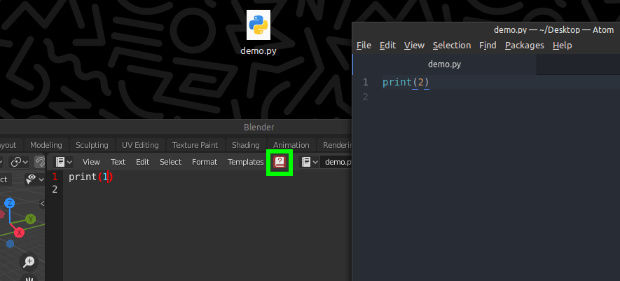
If you click that button, there’s a Reload from disk option; this will update Blender’s Text Editor to reflect the changes you’ve made in your external editor (Atom?). There’s also an option to Make text internal, which saves the Blender version of the script in the .blend file (along with the models, materials, and scene data). I prefer to store Python scripts in separate files so that I have the option of working with code using external tools and switching out scripts as I please.
You can also execute scripts directly from the command line, without having to fully launch Blender. You’ll have to add some code to render the output/visual result, though:
# foo.py
import bpy
bpy.ops.mesh.primitive_cone_add(location=(-3, 0, 0))
output = '/home/nuc/Desktop/render.png'
bpy.context.scene.render.filepath = output
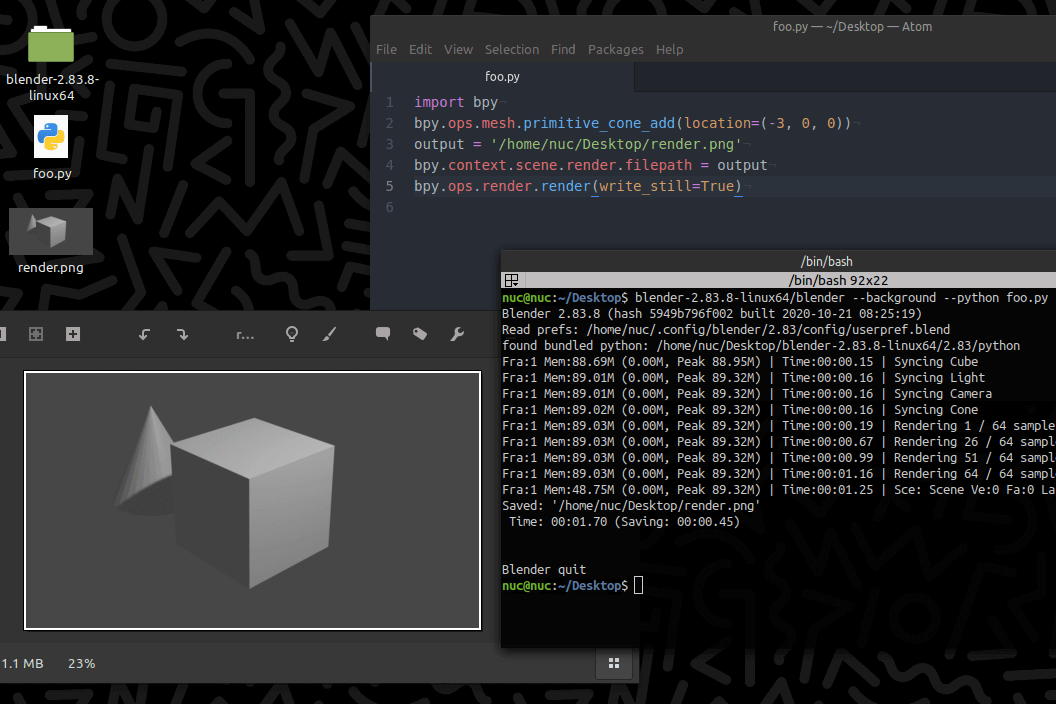
bpy.ops.render.render(write_still=True)This script adds a cone to the standard scene then renders it to a file named render.png (on my Desktop). Note that I’ve also saved the script to my Desktop. To run this, I cd to my Desktop directory and execute the following command:
<blender_dir>/blender --background --python foo.py
Of course, you’ll need to substitute <blender_dir> with the correct path to your blender install. I open the output file (render.png) with an image viewer (Figure 3.12). Most viewers refresh if the image file is updated, so each time I execute the blender command I see the new render.
NOTE: You can press the up arrow key to repeat any command in the terminal.
Better yet, you can additionally configure your code editor to run this command using a keyboard shortcut (rather than the terminal).
If you want a scene with some data you can manipulate, add the .blend file to the command:
<blender_dir>/blender bar.blend --background --python foo.py
The Blender website has more tips and tricks for your coding setup.
Summary
In this short tutorial series, I’ve introduced some Blender scripting fundamentals—the Python Console for one-liners, options you can set to enable Python tooltips and developer extras, the bpy module and some of its attributes and methods, and how to program animation. I also covered some techniques for importing Python code from other files and using external code editors.
But there’s so much to explore in Blender for creative coding. Just about anything you can do in the GUI, you can replicate using Python code, then take that a step further with algorithms you devise. Blender’s Shader Node system is terrific for creating shaders using a visual scripting language (think: connecting nodes as opposed to writing code).
If you’re looking for cool Blender scripts, you can try the following GitHub topic searches: blender-python and blender-scripts. For some inspiring projects, check out: blog.lightprocesses.com; Manu Järvinen’s and Nikolai Janakiev’s Blender scripts; Michael Davies’ spaceship generator. If you’re stuck or have burning technical questions, there’s always Blender’s StackExchange.
If you create anything cool, please share it with me!
End
Complete list of Blender Creative Coding lessons
References
- http://web.purplefrog.com/~thoth/blender/python-cookbook/
- https://blenderscripting.blogspot.com/
- https://docs.blender.org/api/current/
- https://github.com/iklupiani/blenderscriptingwithpython
- https://medium.com/@behreajj